The Jolt Parallelism Problem
Problem Statement
Earlier last week, we
described how changing the set from which we sampled sum-check
challenges could lead 1.3x faster sum-checks. We benchmarked this
optimisation,
and the results were quite conclusive – a particular kind of
multiplication was nearly 2x faster, which could mean binding was
1.3-1.6x faster (accomodating for variance). Furthermore, the empirical
timings from criterion were well aligned with our
theoretical expectations.
So we went ahead an implemented the changes into Jolt, and this led to us changing nearly 145 files, re-design certain parts of Jolt, all so we could manifest this speedup in our end to end traces. We run
cargo run --release -p jolt-core profile --name sha3 --format chrome
and focused on every polynomial bind operation in Jolt1, hoping to see at see at least 5-10% end to end speedup.
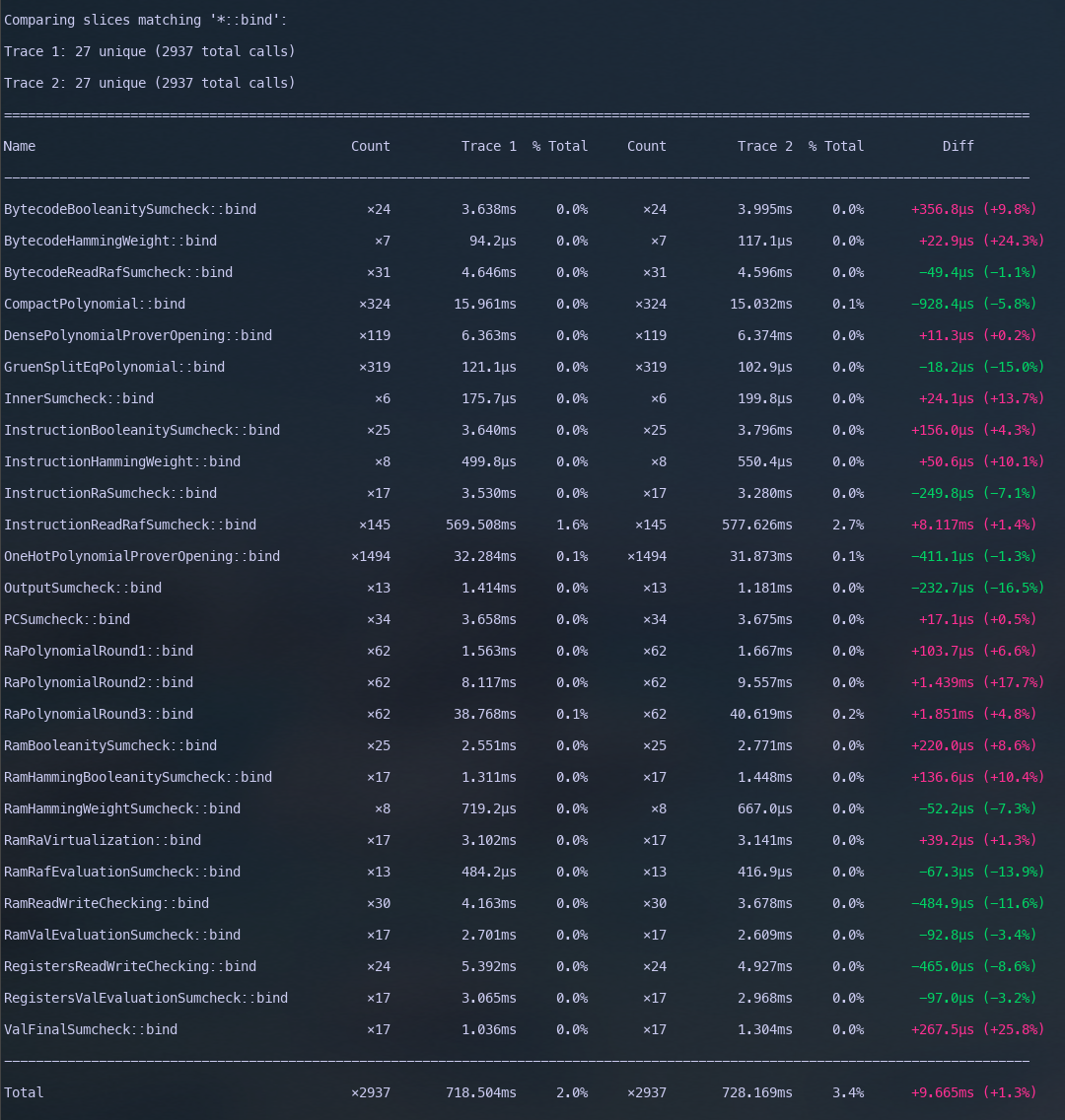
A paltry 1% change in the negative direction. What we see is that essentially, all that extra work made no difference whatsoever. Furthermore, over half of the binding operations in Jolt are slower (or no different) ?? All our micro-benches indicate there should be a speedup, but end to end results indidcate otherwise. The remainder of this post a deep dive into what could possibly the reason for such discrepancy.
Jolt’s Parallelisation Problem
Conjecture: Polynomial binding is an embarrassingly
parallel algorithm. In polynomial binding, we iterate through an array,
and each iteration is independent of the other iterations. This is
exactly the use
case the author of rayon had in mind when
designing the library. So it makes a lot of sense, that Jolt makes heavy
use of rayon for all parallelisation.
Despite rayon’s brilliance, parallel code is incredibly hard to get
right. So as a sanity check we do the following change: We change the
multilinear::bind_parallelto be a sequential algorithm. All
of the binding work gets done in a single thread. Our hope is that end
to end we should slowdown (a lot of binds are sequential), but by
removing the system overhead of parallelism will manifest our low level
optimisations. Remember, the optimisations here are extremely low level.
The difference with base, and our change is roughly 16 mul
instructions. Shown below, is the lines of code we change for this
experiment in the
jolt-core/src/poly/multilinear_polynomial.rs
#[tracing::instrument(skip_all, name = "MultilinearPolynomial::bind_parallel")]
fn bind_parallel(&mut self, r: F::Challenge, order: BindingOrder) {
    match self {
        MultilinearPolynomial::LargeScalars(poly) => poly.bind(r, order),
        MultilinearPolynomial::U8Scalars(poly) => poly.bind(r, order),
        MultilinearPolynomial::U16Scalars(poly) => poly.bind(r, order),
        MultilinearPolynomial::U32Scalars(poly) => poly.bind(r, order),
        MultilinearPolynomial::U64Scalars(poly) => poly.bind(r, order),
        MultilinearPolynomial::I64Scalars(poly) => poly.bind(r, order),
        MultilinearPolynomial::I128Scalars(poly) => poly.bind(r, order),
        MultilinearPolynomial::U128Scalars(poly) => poly.bind(r, order),
        _ => unimplemented!("Unexpected MultilinearPolynomial variant"),
    }
    //match self {
    //    MultilinearPolynomial::LargeScalars(poly) => poly.bind_parallel(r, order),
    //    MultilinearPolynomial::U8Scalars(poly) => poly.bind_parallel(r, order),
    //    MultilinearPolynomial::U16Scalars(poly) => poly.bind_parallel(r, order),
    //    MultilinearPolynomial::U32Scalars(poly) => poly.bind_parallel(r, order),
    //    MultilinearPolynomial::U64Scalars(poly) => poly.bind_parallel(r, order),
    //    MultilinearPolynomial::I64Scalars(poly) => poly.bind_parallel(r, order),
    //    MultilinearPolynomial::I128Scalars(poly) => poly.bind_parallel(r, order),
    //    MultilinearPolynomial::U128Scalars(poly) => poly.bind_parallel(r, order),
    //    _ => unimplemented!("Unexpected MultilinearPolynomial variant"),
    //}
}
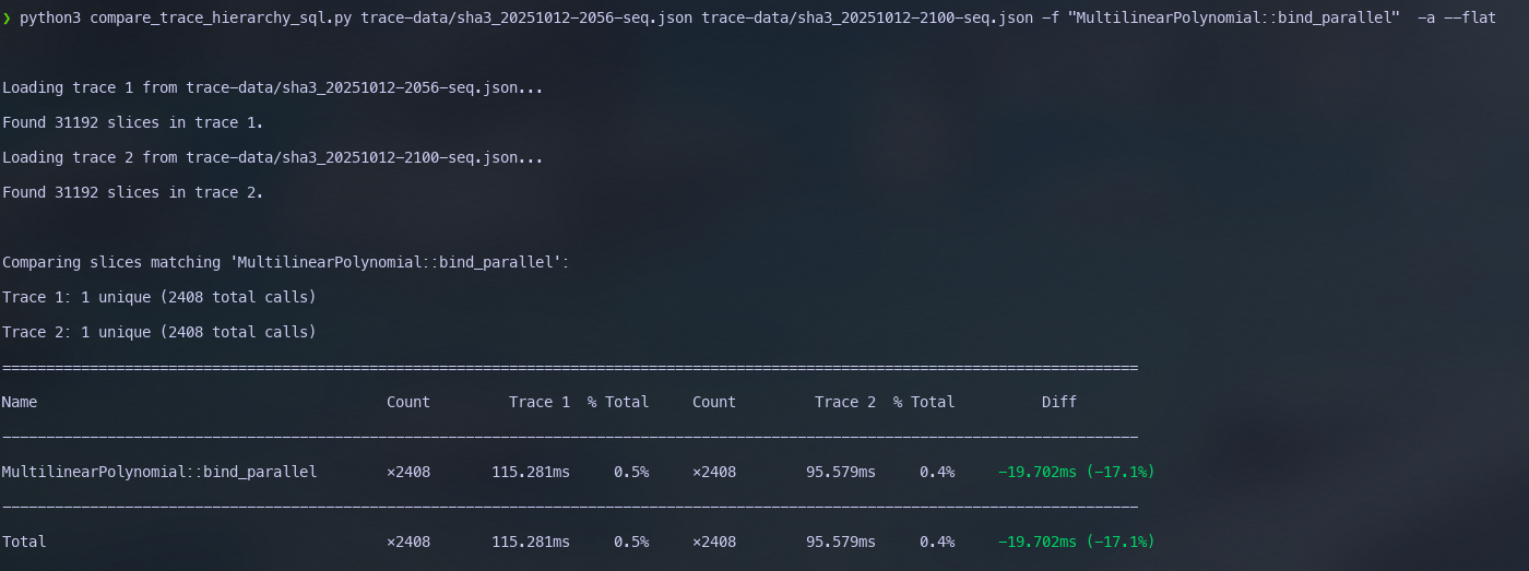
How To Read The Screenshots below
In what follows, unless otherwise stated, Trace 1 will
always refer to running Jolt without small challenges,
and Trace 2 refers to our small challenge optimisation. We
will run both the settings with parallel and sequential binding.
Jolt does not see the benefits of our optimisation.
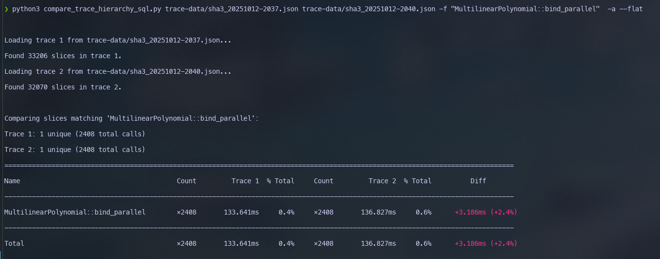
Changing binding to being single threaded leads to 20% empirical
improvement in sum-check binding (aligned with our original
expectations) in the end to end traces. This hints that something fishy
is possibly going on with how we use rayon. Based on the analysis, this number should
be higher than 20% – our micro-benches indicated that this number should
be closer to 40-50%. This 20% loss in performance can be attributed to
caching.
The Actual Problem
Diving deep into what’s actually happening, we show that the issue is not parallelisation, but moreso pure utilisation of cache lines. Our starting point is the following piece of code for binding multi-linear polynomials. From the outset looks perfectly fine, and aligns with exactly what rayon experts would recommend we do.
pub fn bound_poly_var_top_zero_optimized(&mut self, r: &F::Challenge) {
    let n = self.len() / 2;

    let (left, right) = self.Z.split_at_mut(n);

    left.par_iter_mut()
        .zip(right.par_iter())
        .filter(|(&mut a, &b)| a != b)
        .for_each(|(a, b)| {
            *a += *r * (*b - *a);
        });

    self.num_vars -= 1;
    self.len = n;
}
We make one line of change
```rust pub fn bound_poly_var_top_zero_optimized(&mut self, r: &F::Challenge) { let n = self.len() / 2;
let (left, right) = self.Z.split_at_mut(n);

left.par_iter_mut()
    .zip(right.par_iter())
    .with_min_len(4096) // <-- Only change to the code base
    .filter(|(&mut a, &b)| a != b)
    .for_each(|(a, b)| {
        *a += *r * (*b - *a);
});- there is really nothing we can do, parallel code is too hard (possibly, but I am not willing to give in just yet).
So we went ahead and sequentialised the expensive path of the code path. The results are shown below. Unsurprisingly, the overeall bind time is worse. However, it’s only 2x worse.
What’s next
After all this work, the thing that is clear, is nothing is clear. I do not have an definitive answer as what about our use of Rayon nullifies low level multiplication optimisations.
A low hanging fruit is to have a sequential version of every bind, and then check which ones improve the overall end to end speed. This might work in the short term but this is not sustainable. As Jolt evolves and improves, the number of permutations of which binds to keep sequential, and which binds to keep parallel will explode exponentially.
Over the last week, we went ahead studied the Rayon source code. We first outline our working understanding (this will shortly be added) of how Rayon works, with experiments to back up our understanding. A critical feature of
rayonis that it is optimistically parallel. That is to say, given how “work-stealing” is implemented, if the threads are busy, rayon just works like a sequential algorithm, with very minimal overhead. However, our observations described above do not align this claim. Two things are possible – the overhead is really not that minimal (especially, when our optimisations are at the multiplication level, and we are counting assembly instructions). Alternatively, the way we are usingrayonis sub-optimal. There is a third possibility that rayon is not the right tool for Jolt, but I find this highly unlikely.With our working understanding, we have to develop the tools to measure sub-optimal parallelisation. Right now, we can just measure
elapsed time. We need to look at cpu counters, andstracereports to see how often the threads are spinning, or if there are stragglers. Perhaps we can implement some dynamic instrumentation to focus our CPU counter collection only during some functions. This gives us a much clearer picture as to how multi-threading could be a bottleneck.
The figures are generated using jolt-perfetto, a light wrapper on top of trace_processor shell.↩︎