Smaller Sumcheck Challenges In Jolt
TL;DR - Just Tell Us What You Did
Faster Sumcheck In Jolt
By sampling the verifiers random challenges from a set \(S \subset \mathbb{F}\) of size roughly \(\sqrt{|\mathbb{F}|}\), we speed up sum-check binding by 1.6x from baseline (where challenges are sampled over the whole field \(\mathbb{F}\) – the field over which polynomials are defined. )
NOTE: This now reduces the soundness error from
\(1/2^{254}\) to \(1/2^{125}\), but this is not a concern as
currently Jolt usess the bn256 curve to commit to
polynomials, which offers 110 bits of security anyway.
What does this mean for end to end performance? – We’ve sped up sum-check, that should speed up everything right? The answer is Yes – in theory, but we cannot yet materialise these improvements in our end to end system. The reason why, has nothing to do with the optimisations we are going to discuss below. A short description of the reason is – our parallelisation code is not perfect – this prevents our traces from always accurately reflecting the impact of low level optimisations (especially optimisations that are in the thick of parallel code). We are in the process of writing a detailed report of this issue. When it’s ready, it’ll be available here.
With that said, here’s are the details of how we came up with this optimisation. First we briefly review the sum-check protocol, which prepares us to understand exactly why speeding up a certain type of multiplication would be beneficial. Then we get to showing how we speed up the multiplication, and end with benches that confirm theory.
Sum-Check Recap
We briefly recap the sum-check protocol1.
Let \(g \in \mathbb{F}[X_1, \ldots, X_m]\) be a polynomial over \(\mathbb{F}\) with the following structure. \[ g(X_1, \ldots, X_m) = \prod_{j=1}^d q_j(X_1, \ldots, X_m)\] where all \(q_j(X)\)’s are multi-linear polynomials over \(\mathbb{F}\). > > > > > > > We expand more below:
- Polynomial evaluation The prover computes the following univariate polynomial, using the following steps \[p_i(X_i) = \sum_{b_{i+1} \in \{0,1\}}\ldots\sum_{b_{m} \in \{0,1\}^{}}g(r_1, \ldots, r_{i-1}, X_i, b_{i+1}, b_m)\]
- If \(g\) has degree \(d\), this requires computing \(p_i(0), \ldots, p_i(d)\), then via standard lagrange interpolation, we’re able to fully define \(p_i(X)\). \[p_i(Z) = \prod_{j=1}^d \Bigg( \sum_{b_{i+1} \in \{0,1\}}\ldots\sum_{b_{m}} q_j\Big(r_1, \ldots, r_{i-1}, Z, b_{i+1}, \ldots, b_m\Big)\Bigg)\] so to get \(p_i(Z)\) we compute for all \(j \in [d]\), \(q_j(r_1, \ldots, r_{i-1}, Z, \vec{b})\) for \(Z \in \{0, \ldots, d\}\) for all \(\vec{b} \in \{0, 1\}^{m-i}\). As \(q_j\) is multi-linear – this can be computed by linear-interpolation.
\[ \begin{aligned} q_j(r_1, \ldots, r_{i-1}, Z, \vec{b}) = & (1-Z) \,q_j(r_1, \ldots, r_{i-1}, 0, b_{i+1}, \ldots, b_m) \\[10pt] & + Z\, q_j(r_1, \ldots, r_{i-1}, 1, b_{i+1}, \ldots, b_m) \end{aligned} \]
As \(d\) is a small constant number, computing the above value requires no multiplication operations. We can compute it via a running sum. See pseudocode below
/// Compute q_j(Z) = (1-Z) * q_j(0) + Z * q_j(1)
/// using only additions
/// when Z is a small integer.
    fn compute_q_j_running_sum(z: usize, q_at_0: JoltField, q_at_1: JoltField) -> JoltField {
        let diff = q_at_1 - q_at_0;

        // Compute Z * diff using repeated addition (running sum)
        let mut z_times_diff = JoltField::zero();
        for _ in 0..z {
            z_times_diff += diff;
        }

        q_at_0 + z_times_diff

    }
Binding Phase Thee prover needs to binds the multi-linear polynomial \(g\) to \(r_i\), that is to say it computes a new multi-linear polynomial in \(m-i\) variables \[g_i(X_{i+1}, \ldots, X_{m}) = g(r_1, \ldots, r_{i-1}, X_{i+1}, \ldots, X_{m})\]. This involves storing all evaluations of \(g_i\) over the hyper cube \(\{0, 1\}^{m-i}\), but unlike the above step \(r_i\) is NOT guaranteed to be a small number. Therefore the running sum described in the pseudocode above is no good to use. We need to use actual multiplication here.
\[\begin{aligned} q_j(r_1, \ldots, r_{i-1}, \textcolor{orange}{r_i}, \vec{b}) = & (1-\textcolor{orange}{r_i}) \,q_j(r_1, \ldots, r_{i-1}, 0, b_{i+1}, \ldots, b_m) \\[10pt] & + \textcolor{orange}{r_i}\, q_j(r_1, \ldots, r_{i-1}, 1, b_{i+1}, \ldots, b_m) \end{aligned}\]$$
Now \(q_j(r_1, \ldots, r_{i-1}, 1, b_{i+1}, \ldots, b_m) \in \mathbb{F}\), and traditionally the set \(S\) from which we sample \(r_i\) is also equal to \(\mathbb{F}\). Therefore this step requires \(2^{m-i}\) \(\mathbb{F}\times \mathbb{F}\) multiplications in round \(i\) – a total of \(2^m\) multiplications over \(m\) rounds. It is well known that multiplication for \(\mathbb{F}\) elements is 1000x costlier than addition. So our hope is that we can choose \(S\) cleverly such that this operation can be done faster. Note we cannot make \(S\) too small, as this the soundness probability of any sumcheck protocol is given by \(\frac{d}{|S|}\).
What we show
We show that there exists a set \(S\) of size rouhgly \(|\mathbb{F}|^{1/2}\), which we call
MontU128Challenge, in which \(\mathbb{F}\times r\) is 1.6x faster than
\(\mathbb{F}\times \mathbb{F}\). This
in returns speeds up the binding phase of the sum-check
protocol, which results in a 1.3x speedup per round of sum-check.
The Challenge Set \(S\)
Define the set
\[ S \subset \mathbb{F}\text{where} S = \{ x \in \mathbb{F}: \text{the least 2 significant digits of $x$ in Montgomery form are 0} \} \]
Worked Out Example:
Prime Field \(\mathbb{F}= \mathbb{Z}_{13}\) with Montgomery Form. Montgomery parameter: \(R = 16 = 2⁴\). Montgomery form of \(x\) is given by \(xR \mod 13\)
| x | Montgomery Form (decimal) | Binary | Last 2 bits |
|---|---|---|---|
| 0 | 0 | 0000 | 00 ✓ |
| 1 | 3 | 0011 | 11 |
| 2 | 6 | 0110 | 10 |
| 3 | 9 | 1001 | 01 |
| 4 | 12 | 1100 | 00 ✓ |
| 5 | 2 | 0010 | 10 |
| 6 | 5 | 0101 | 01 |
| 7 | 8 | 1000 | 00 ✓ |
| 8 | 11 | 1011 | 11 |
| 9 | 1 | 0001 | 01 |
| 10 | 4 | 0100 | 00 ✓ |
| 11 | 7 | 0111 | 11 |
| 12 | 10 | 1010 | 10 |
\[S = \{0, 4, 7, 10\}\]
Note: \(|S| = 4 \approx \sqrt{p}\), which makes sense since we’re filtering by the last 2 bits.
The short answer to why we this set \(S\) is nice, is that it saves us 10 multiplication instructions per field multiplication. We first briefly review the CIOS algorithm, which is currently used to multiply field elements.
CIOS Review
Let \(n\) be the number of limbs used to represent field elements. Currently in Jolt, \(n=4\). The width \(w\) of each limb is 64 bits. Given \(a \in \mathbb{F}\) and \(b\in S\) , let \(\widetilde{a} = aR \mod p, \widetilde{b} = bR \mod p\) be the respective Montgomery representations.
Let \(c = \widetilde{a}\widetilde{b}\) computed using textbook limb by limb multiplication. Now to get \(\widetilde{c}\) we need to compute \(cR^{-1} = cr^{-n} = (ab)R \mod p\).
\(c\) can be written as the following sum and we compute \(cR^{-1}\) limb by limb by multiplying \(r^{-1}\) \(n\) times
\[ \begin{align} c & \equiv (c_{2n-1} r^{2n-1} + c_{2n-2} r^{2n-2} + \ldots + c_1r + c_0) \mod p \\[10pt] cr^{-1} & \equiv ( c_{2n-1}r^{2n-1} + c_{2n-2} r^{2n-2} + \ldots + c_1r)r^{-1} + c_0 r^{-1} \mod p \\[10pt] \end{align} \]
Important Sub-Routine
Observe that \(c_0r^{-1} \equiv (c_0 + mp)r^{-1} \mod p\), where \(m\) such that \(c_0 + mp \equiv 0 \mod r\). Solving for \(m = -p^{-1}c_0 \equiv \mu c_0 \mod r\). Also as we are working modulo \(r\), it suffices to use \(m = \mu_{0}c_0\) discarding any carries, where \(\mu_{0}\) is the least significant word of \(\mu\).
Once we compute \(mp\), and add this to \(c\) to get \(c^{(1)}\), this should clear the least significant digit based on how we picked \(m\). See below
\[ \begin{align} c & \equiv (c_{2n-1} r^{2n-1} + c_{2n-2} r^{2n-2} + \ldots + c_1r + c_0) \mod p \\[10pt] cr^{-1} & \equiv ( c_{2n-1}r^{2n-1} + c_{2n-2} r^{2n-2} + \ldots + c_1r)r^{-1} + c_0 r^{-1} \mod p \\[10pt] & \equiv ( c_{2n-1}r^{2n-1} + c_{2n-2} r^{2n-2} + \ldots + c_1r)r^{-1} + (c_0+ mp)r^{-1} \mod p \\[10pt] & \equiv (c + mp)r^{-1} \mod p \\[10pt] & \equiv ( c^{(1)}_{2n-1}r^{2n-1} + \ldots c^{(1)}_1r + 0)r^{-1} \mod p \\[10pt] & \equiv ( c^{(1)}_{2n-1}r^{2n-2} + \ldots c^{(1)}_1) \mod p \\[10pt] \end{align} \]
Repeat The Subroutine \(n\) times
Now we can play the subroutine again with \(c^{(1)}_1\) replacing the role of \(c_0\), and the updated value of \(m = \mu_0c_1^{(1)}\) (NOTE the same \(\mu_0\) is always used)
\[ \begin{align} cr^{-1} & \equiv ( c^{(1)}_{2n-1}r^{2n-2} + \ldots c^{(1)}_1 ) \mod p \\ cr^{-2} & \equiv ( c^{(1)}_{2n-1}r^{2n-3} + \ldots + c_1^{(1)}+ c_1^{(1)}r^{-1} \mod p \\ & \equiv ( c^{(2)}_{2n-1}r^{2n-3} + \ldots + c_1^{(2)} ) \mod p \end{align} \]
In fact we play this game \(n\) times
\[cR^{-1} \equiv cr^{-n} \equiv c^{(n)}_{2n-1}r^{n-1} + c^{(n)}_{n+1}r +c^{(n)}_{n} \mod p\]
To get the final answer2
Total Multiplications
The total number of multiplications is \(2n^2 + n\) which for \(n=4\) is 36.
- \(n^2\) multiplications to compute \(c\).
- \(n\) multiplications to compute to \(m=\mu_i c_i^{(i)}\) in each round.
- \(n\) multiplications to compute \(mp\) per round which totals \(n^2\) multiplications.
Next we illustrate how sampling \(\widetilde{b} \xleftarrow[]{\$}S\) saves us multiplications.
Firstly when 2 digits are 0 we we only need \(n \times (n-2)\) multiplications, which allows us to save 8 multiplications when \(n=4\).

Remember the reduction phase is all about 0’ing out the least significant digit. If it’s already 0 we do not need to compute \(m_0 p\) and \(m_1p\) anymore.

This saves us \(8 + 2 + 8= 20\) multiplications, which leaves with only \(16\) multiplications
If multiplications were the only thing that cost us CPU cycles we should see roughly 2x speedup. However, additions and bit shifts – although significantly cheaper, are not free. Thus, a reasonable expectation would be to see 1.6-1.8x speedup.
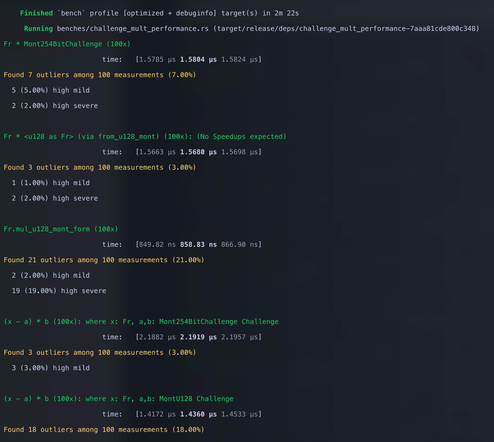
So we compute \((a-b)\times c\), where \(a,b\in\mathbb{F}\) and \(c\in S\), 100 times and measure how long it takes.
- \(S = \mathbb{F}\)
- \(S\) is 2 least significant digits 0’d out.
cargo bench -p jolt-core --bench challenge_mult_performance
Next we show that this improved multiplication does indeed speed up polynomial binding
cargo bench -p jolt-core --bench binding
cargo bench -p jolt-core --bench binding --features challenge-254-bit
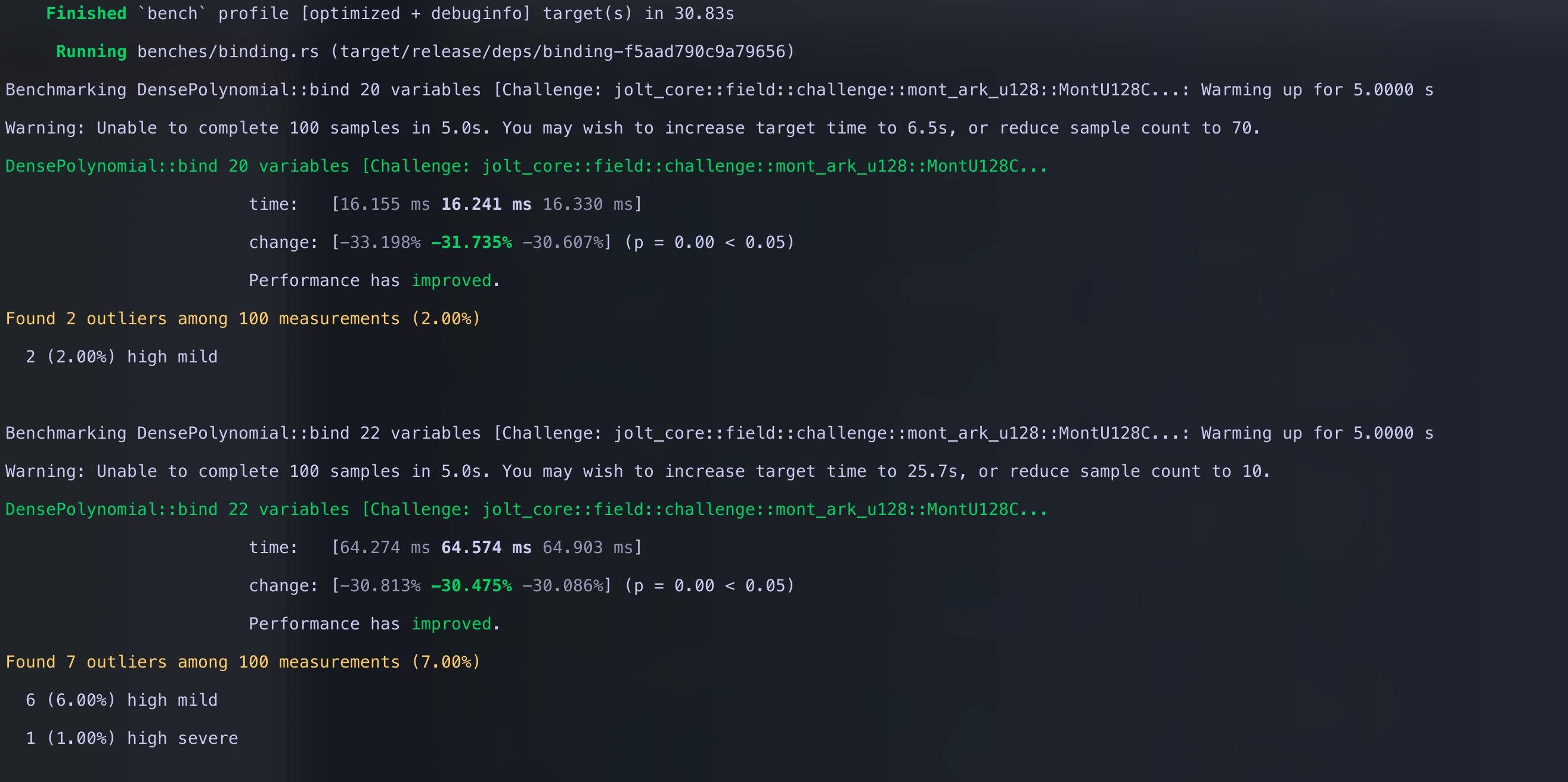 Comparing
it against the baseline
Comparing
it against the baseline
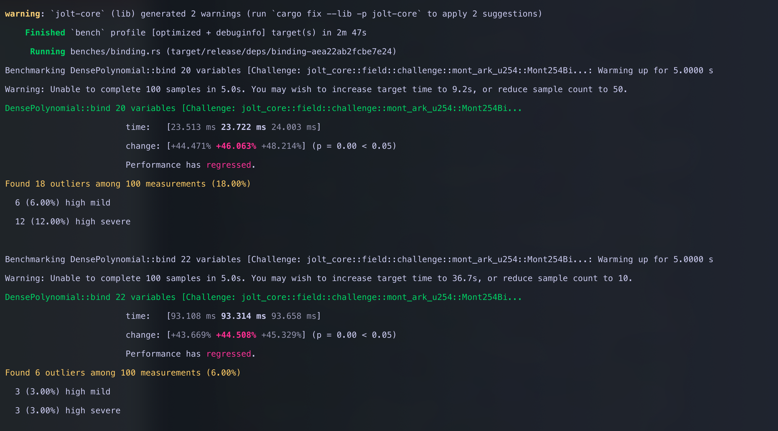
Shown below is the diff from bench with the red pdf representing our fast multiplication.

Some Implementation Details
we use \(256\) bits to represent big
integers and our challenge and the modulus for ark-bn256
uses \(254\) bits. Thus, if sampled a 2
limbed \(128\) bit integer \(x\) and used that as the challenge as is
x = [x_1, x_0, 0, 0] we are not guaranteed that \(x < p\) which the CIOS algorithm
assumes. we use \(256\) bits to
represent big integers and our challenge and the modulus for
ark-bn254 uses \(254\)
bits. Thus, if sampled a 2 limbed \(128\) bit integer \(x\) and used that as the challenge as is
x = [x_1, x_0, 0, 0] we are not guaranteed that \(x < p\) which the CIOS algorithm
assumes. So we clear the first 3 bits of \(x\) to ensure that \(x\) is ALWAYS less than
\(p\).
impl<F: JoltField> MontU128Challenge<F> {
pub fn new(value: u128) -> Self {
    // MontU128 can always be represented by 125 bits.
    // This guarantees that the big integer is never greater than the
    // bn254 modulus
    let val_masked = value & (u128::MAX >> 3);
    let low = val_masked as u64;
    let high = (val_masked >> 64) as u64;
    Self {
        value: [0, 0, low, high],
        _marker: PhantomData,
    }
}

pub fn value(&self) -> [u64; 4] {
    self.value
}

pub fn random<R: Rng + ?Sized>(rng: &mut R) -> Self {
        Self::from(rng.gen::<u128>())
    }
}
The actual multiplication is in the A16z fork of
arkworls-algebra crate.
Below is a snippet of the optimised CIOS code for the set \(S\) above
Footnotes and References
There are optimisations by [?] that improve on this, but the optimisations discussed in this note still apply, so for the sake of simplicity, we describe the Sum-check protocol in its simplest form.↩︎
We have to conditionally subtract from \(p\) to get the actual right answer, but this operation is common to both the baseline and our optimisation, so we do not focus on this.↩︎