Faster Polynomial Evaluaton

Tracked Data Types

Before, describing optimisations to polynomial evaluation, we discuss an additional tool to debug numerical algebra libraries. In Jolt sum-check algorithms, almost invariably the bottleneck in computation is number of field multiplications by large scalars. So it might be helpful to be able to count the number of multiplications your algorithm does, and check if we’re under the theoretical limit.

Towards this we introduce TrackedFr data type which is exactly the same as ark_bn254::Fr except for 1 critical difference. Implementation here

Before performing a multiplication operation, we increment a global counter atomically (in a thread safe way). Rust makes this relatively easy to do (it’s remarkable how far libraries have come that prevent us from writing semaphores and mutexes from scratch) See [official docs here]](https://doc.rust-lang.org/std/sync/atomic/struct.AtomicUsize.html)

use std::sync::atomic::{AtomicUsize, Ordering};

  // A global counter that tracks how many times we've use a*b where a, b are ark_bn254::Fr types
  // see jolt-core::field::tracked_fr::TrackedFr for more details
  pub static MULT_COUNT: AtomicUsize = AtomicUsize::new(0);
  

We have the ability to reset this counter at any time as well. So now all we need to do if we wanted to see how many multiplications transpired, is to wrap the function being examined with reset_mult_count() and get_mult_count(). See an example of how to use here.

That’s it! Right now it just tracks multiplications, but you may extend it to any operation ark_bn254::Fr does by simply wrapping the operation as follows:

For all types of multiplication we do w

// crate is jolt-core
  use crate::utils::counters::MULT_COUNT;

  // Owned * owned
  impl Mul<TrackedFr> for TrackedFr {
      type Output = TrackedFr;
      fn mul(self, rhs: TrackedFr) -> Self::Output {
          MULT_COUNT.fetch_add(1, Ordering::Relaxed);
          TrackedFr(self.0 * rhs.0)
      }
  }

  // Owned * borrowed
  impl<'a> Mul<&'a TrackedFr> for TrackedFr {
      type Output = TrackedFr;
      fn mul(self, rhs: &'a TrackedFr) -> Self::Output {
          MULT_COUNT.fetch_add(1, Ordering::Relaxed);
          TrackedFr(self.0 * rhs.0)
      }
  }

  // Borrowed * owned
  impl Mul<TrackedFr> for &TrackedFr {
      type Output = TrackedFr;

      fn mul(self, rhs: TrackedFr) -> Self::Output {
          MULT_COUNT.fetch_add(1, Ordering::Relaxed);
          TrackedFr(self.0 * rhs.0)
      }
  }

  #[allow(clippy::needless_lifetimes)]
  impl<'a, 'b> Mul<&'b TrackedFr> for &'a TrackedFr {
      type Output = TrackedFr;
      fn mul(self, rhs: &'b TrackedFr) -> Self::Output {
          MULT_COUNT.fetch_add(1, Ordering::Relaxed);
          TrackedFr(self.0 * rhs.0)
      }
  }

Problem Statement

Fix \(n \in \mathbb{N}\) and define \(N = 2^n\). In the Jolt codebase there is an algorithm that takes as input a vector \(f \in \mathbb{F}^N\) and an \(\vec{z} \in \mathbb{F}^n\) and outputs \(\widetilde{f}(\vec{z})\) where \(\widetilde{f}\) is the multilinear extension (MLE) of \(f\). See Chapter 3 of (Thaler, 2020) for details on how to compute MLE of a vector.

More specifically, the current algorithm does the following:

1. Given \(\vec{z} \in \mathbb{F}^n\) it computes all \(N = 2^n\) evaluations of Lagrange basis polynomials \(\Big\{\chi_{\vec{w}}(\vec{z})\Big\}_{\vec{w} \in \{0,1 \}^n}\) where \(\chi_{\vec{w}}(\vec{z}) = \prod_{k=1}^{n} (1 -z_k)(1-w_k) + z_k w_k = eq(\vec{w}, \vec{z})\).

Using the memoization algorithm described in (Vu et al., 2013), this computation require \(N\) multiplications. See Lemma 3.8 of (Thaler, 2020) for a simple exposition and analysis of this algorithm. An implementation can be found here.

2. Then to compute the answer we compute a dot product, which requires \(N\) multiplications. \[\widetilde{f}(\vec{z}) = \sum_{w \in \{0,1\}^n}f(w)\chi_{\vec{w}}(\vec{z})\]

In what follows, we describe how to speed up the implementation by a factor of 2.

A Constant Factor Improvement

Re-writing the definition of MLE of \(f\) we get \[ \begin{align} \widetilde{f}(\vec{z}) &= \sum_{\vec{w} \in \{0,1\}^n}f(w)\cdot \chi_{\vec{w}}(\vec{z})\\[10pt] &=\sum_{\vec{w} \in \{0,1\}^n} f(\vec{w})\cdot eq(\vec{z},\vec{w}) \\[10pt] &= \sum_{w_1 \in \{0,1\} } eq(z_1,w_1) \sum_{w_2 \in \{0,1\} } eq(z_2,w_2) \ldots \sum_{w_n \in \{0, 1\}} eq(z_n,w_n) * f(w_1,...,w_n) \end{align} \]

Notice that for any \((w_1, \ldots, w_{n-1}) \in \{ 0, 1\}^{n-1}\) \[ \begin{align} \sum_{w_n \in \{0,1\}} \operatorname{eq}(z_n, w_n) \cdot f(w_1, \ldots, w_n) &= f(w_1, \ldots, w_{n-1}, 0) \notag \\ &\quad + z_n \cdot \left( f(w_1, \ldots, w_{n-1}, 1) - f(w_1, \ldots, w_{n-1}, 0) \right) \end{align} \]

which is one multiplication for every instantiation of \((w_1, \ldots, w_{n-1})\), therefore it is a total of \(2^{n-1}\) multiplications.

Now if we compute things inside out i.e \(j \in \{n, \ldots, 1\}\),

• The first iteration of the loop is \(2^{n-1}\) multiplications
• The second iteration will be \(2^{n-2}\) multiplications
• …
• The \(j\)’th itertion will be \(2^{n-j}\) multiplications
• …
• The last iteration is just 1 multiplication.

Thus, there is a total of \(N =2^n\) multiplications, instead of the two step process described above, each of which had \(2N\) multiplications aove

Leveraging Sparsity

Now what if told you that \(\gamma\) fraction of the evaluations of \(\widetilde{f}\) over \(\{0, 1\}^n\) are zero. Then the dot product implementation requires :

• \(N + \gamma N\) multiplications.

An alternative way to implement this dot product algorithm is take \(\vec{z} = \vec{z_1} || \vec{z_2}\) and split into 2 halves of size \(n/2\) and compute

\[\sum_{\vec{x_1} \in \{ 0, 1\}^{n/2}}\mathsf{eq}(\vec{z_1}, \vec{x_1})\sum_{\vec{x_2} \in \{ 0, 1\}^{n/2}}eq(\vec{z_2}, \vec{x_2})\widetilde{f}(x_1||x_2)\]

This takes

• \(2\sqrt{N} + \sqrt{N} + \gamma N = 3\sqrt{N} + \gamma N\) multiplications

The inside-out evaluation, also leverages sparsity, but in a way that depends on the distribution of 0s. Imagine \(N=8\) and the following two arrays

[12, 32, 55, 121, 0, 0, 0, 0]
  [0, 32, 55, 0, 0, 21, 11, 0]

In the first case, despite having half the evaluations set to 0, \(z(f[i] - f[m2+i])\) is not zero. in the second case, the zero’s align well and we can get rid of two out of 4 multiplications.

Below are two plots that show the impact of sparsity on a single polynomial evaluation. The plot on top shows exactly how many multiplications are occurring for each algorithm (note dot_product is not checking for zeros, so it’s \(2N\) always). Also shown in a dashed line is the theoretical upper bound for the algorithm that spilts eq, and this confirms that our implementation is efficient,

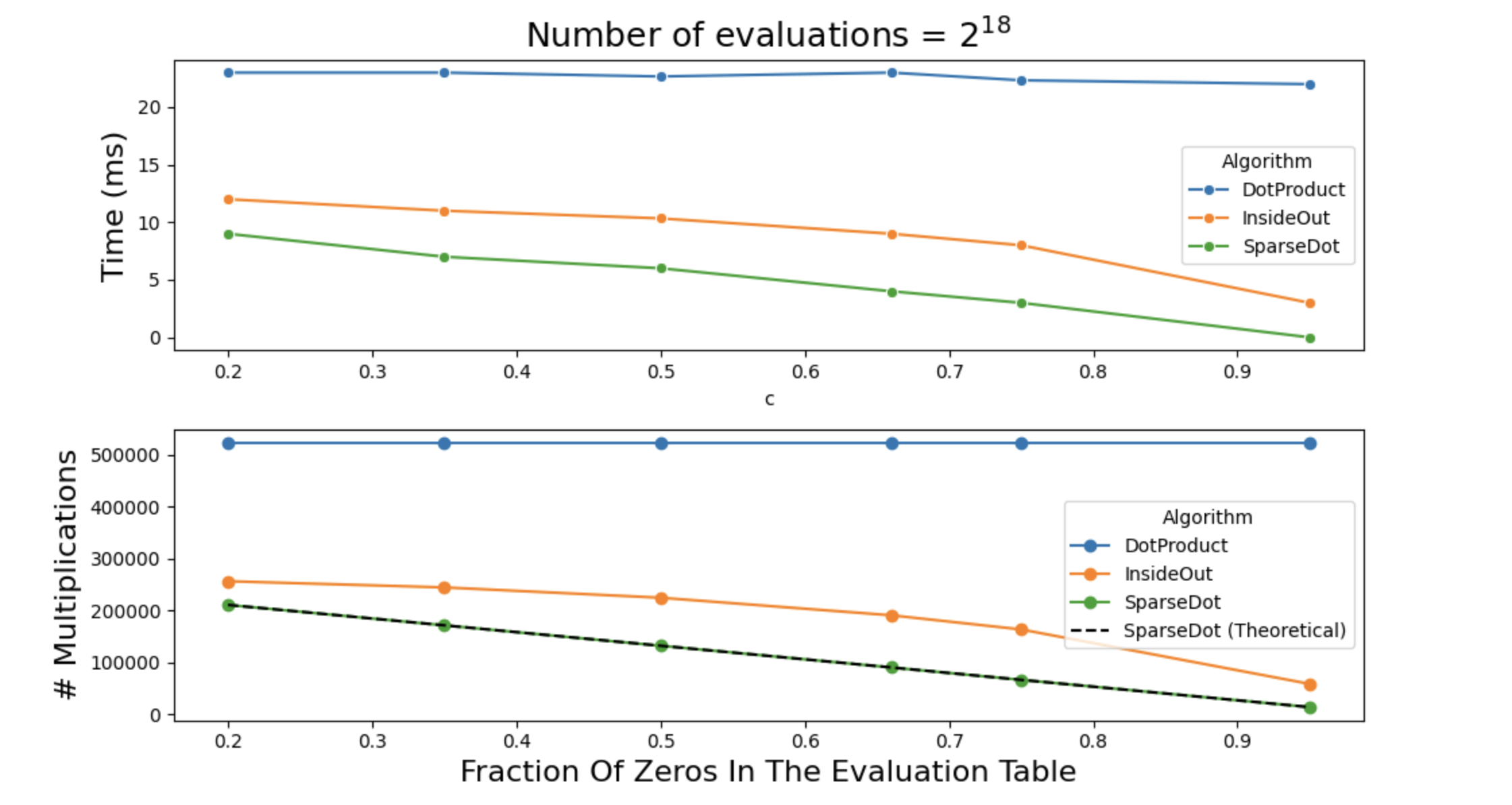
The plot below shows the physical times. Notice how the two trends are almost identical, which does confirm that the bottleneck in polynomial evaluation really is field multiplication.

How to get these plots yourself:

cargo run -p jolt-core --example polynomial_evaluation --release

This should generate a file called results.csv from which the above numbers can be easily calculated.

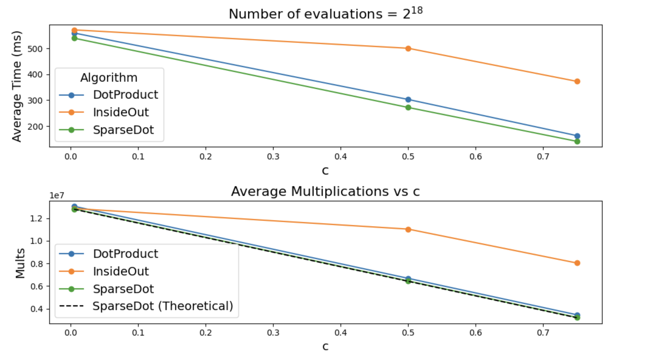
Batched Polynomial Evaluation

Now we get to batched evaluations, that is we want to evaluate multilinear polynomials \(f_1, \ldots, f_s\) at the same point \(\vec{z}\).

Now the cost of computing \(eq\) is not as bad as it can be re-used for all \(\{f_i\}_{i \in [s]}\). Still we show splitting \(eq\) into \(eq_1\) and \(eq_2\) can provide time savings.

Once again we will measure both the exact number of multiplications, and the actual time it took to multiply things.

To get these plots run

cargo run -p jolt-core --example polynomial_evaluation --release

and you shall receive a file called batch_results.csv