Faster Polynomial Evaluaton
Problem Statement
Fix \(n \in \mathbb{N}\) and define \(N = 2^n\). :In the Jolt codebase there is an algorithm that takes as input a vector \(f \in \mathbb{F}^N\) and an \(\vec{z} \in \mathbb{F}^n\) and outputs \(\widetilde{f}(\vec{z})\) where \(\widetilde{f}\) is the multilinear extension (MLE) of \(f\). See Chapter 3 of (Thaler 2020) for details on how to compute MLE of a vector.
More specifically, the current algorithm does the following:
- Given \(\vec{z} \in \mathbb{F}^n\) it computes all \(N = 2^n\) evaluations of Lagrange basis polynomials \(\Big\{\chi_{\vec{w}}(\vec{z})\Big\}_{\vec{w} \in \{0,1 \}^n}\) where \(\chi_{\vec{w}}(\vec{z}) = \prod_{k=1}^{n} (1 -z_k)(1-w_k) + z_k w_k = eq(\vec{w}, \vec{z})\).
Using the memoization algorithm described in (Vu et al. 2013), this computation require \(N\) multiplications. See Lemma 3.8 of (Thaler 2020) for a simple exposition and analysis of this algorithm. An implementation can be found here.
- Then to compute the answer we compute a dot product, which requires \(N\) multiplications. \[\widetilde{f}(\vec{z}) = \sum_{w \in \{0,1\}^n}f(w)\chi_{\vec{w}}(\vec{z})\]
In what follows, we describe how to speed up the implementation by a factor of 2.
A Constant Factor Improvement
Re-writing the definition of MLE of \(f\) we get
\[ \begin{align} \widetilde{f}(\vec{z}) &= \sum_{\vec{w} \in \{0,1\}^n}f(w)\cdot \chi_{\vec{w}}(\vec{z})\\[10pt] &=\sum_{\vec{w} \in \{0,1\}^n} f(\vec{w})\cdot eq(\vec{z},\vec{w}) \\[10pt] &= \sum_{w_1 \in \{0,1\} } eq(z_1,w_1) \sum_{w_2 \in \{0,1\} } eq(z_2,w_2) \ldots \sum_{w_n \in \{0, 1\}} eq(z_n,w_n) * f(w_1,...,w_n) \end{align} \]
Notice that for any \((w_1, \ldots, w_{n-1}) \in \{ 0, 1\}^{n-1}\)
\[ \begin{align} \sum_{w_n \in \{0,1\}} \operatorname{eq}(z_n, w_n) \cdot f(w_1, \ldots, w_n) &= f(w_1, \ldots, w_{n-1}, 0) \notag \\ &\quad + z_n \cdot \left( f(w_1, \ldots, w_{n-1}, 1) - f(w_1, \ldots, w_{n-1}, 0) \right) \end{align} \]
which is one multiplication for every instantiation of \((w_1, \ldots, w_{n-1})\), therefore it is a total of \(2^{n-1}\) multiplications.
Now if we compute things inside out i.e \(j \in \{n, \ldots, 1\}\),
- The first iteration of the loop is \(2^{n-1}\) multiplications
- The second iteration will be \(2^{n-2}\) multiplications
- …
- The \(j\)’th itertion will be \(2^{n-j}\) multiplications
- …
- The last iteration is just 1 multiplication.
Thus, there is a total of \(N =2^n\) multiplications, instead of the two step process described above, each of which had \(2N\) multiplications aove
Fully Worked Out Example For Inside Out Algorithm
Notation: Bits are written in BigEndian where the left most bit is the MSB.
Given all evaluations of multi-linear polynomial \(f\)
\[ \begin{aligned} f(0, 0, 0) &= 0 \\ f(0, 0, 1) &= 0 \\ f(0, 1, 0) &= 1 \\ f(0, 1, 1) &= 0 \\ f(1, 0, 0) &= 0 \\ f(1, 0, 1) &= 0 \\ f(1, 1, 0) &= 0 \\ f(1, 1, 1) &= 1 \end{aligned} \]
We are told to compute \(f(4, 3, 2)\),
Step 1
\[ \begin{align*} f(0, 0, 2) &= f(0, 0, 0) + 2(f(0, 0, 1) - f(0, 0, 0)) &= 0 + 2(0 - 0) &= 0 \\ f(0, 1, 2) &= f(0, 1, 0) + 2(f(0, 1, 1) - f(0, 1, 0)) &= 1 + 2(0 - 1) &= -1 \\ f(1, 0, 2) &= f(1, 0, 0) + 2(f(1, 0, 1) - f(1, 0, 0)) &= 0 + 2(0 - 0) &= 0 \\ f(1, 1, 2) &= f(1, 1, 0) + 2(f(1, 1, 1) - f(1, 1, 0)) &= 0 + 2(1 - 0) &= 2 \end{align*} \]
Step 2:
\[ \begin{align*} f(0, 3, 2) &= f(0, 0, 2) + 3(f(0, 1, 2) - f(0, 0, 2)) &= 0 + 3(-1 - 0) &= -3 \\ f(1, 3, 2) &= f(1, 0, 2) + 3(f(1, 1, 2) - f(1, 0, 2)) &= 0 + 3(2 - 0) &= 6 \end{align*} \]
Step 3
\[ \begin{align*} f(4, 3, 2) &= f(0, 3, 2) + 4(f(1, 3, 2) - f(0, 3, 2)) \\ &= -3 + 4(6 - (-3)) = -3 + 4 \cdot 9 = -3 + 36 = \boxed{33} \end{align*} \]
Leveraging Sparsity
Now what if told you that \(\gamma\) fraction of the evaluations of \(\widetilde{f}\) over \(\{0, 1\}^n\) are zero. Then the dot product implementation requires :
- \(N + \gamma N\) multiplications.
The current
Jolt Implementation did not leverage sparsity at all. That is even
multiplying a*b it does not check if a or
b is zero to simply return 0. It goes ahead and does
montgomery multiplication anyway, which is wasteful.
This is not the case with batched evaluation we will discuss
later which uses 01_optimised_multo get rid of this
inefficiency. Code:
.
An alternative way to implement this dot product algorithm is take \(\vec{z} = \vec{z_1} || \vec{z_2}\) and split into 2 halves of size \(n/2\) and compute
\[\sum_{\vec{x_1} \in \{ 0, 1\}^{n/2}}\widetilde{\mathsf{eq}}\left((, \vec \right){z_1}, \vec{x_1})\sum_{\vec{x_2} \in \{ 0, 1\}^{n/2}}eq(\vec{z_2}, \vec{x_2})\widetilde{f}(x_1||x_2)\]
This takes
- \(2\sqrt{N} + \sqrt{N} + \gamma N =
3\sqrt{N} + \gamma N\) multiplications as opposed to the \(N + \gamma N\) approach taken by
01_optimised_muldiscussed above.
The inside-out evaluation, also leverages sparsity, but in a way that depends on the distribution of 0s. Imagine \(N=8\) and the following two arrays
[12, 32, 55, 121, 0, 0, 0, 0]
[0, 32, 55, 0, 0, 21, 11, 0]
In the first case, despite having half the evaluations set to 0, \(z(f[i] - f[m/2+i])\) is not zero. in the second case, the zero’s align well and we can get rid of two out of 4 multiplications.
Below are two plots that show the impact of sparsity on a single
polynomial evaluation. The plot on top shows exactly how many
multiplications are occurring for each algorithm (note
dot_product is not checking for zeros, so it’s \(2N\) always). Also shown in a dashed line
is the theoretical upper bound for the algorithm that spilts
eq, and this confirms that our implementation is
efficient.
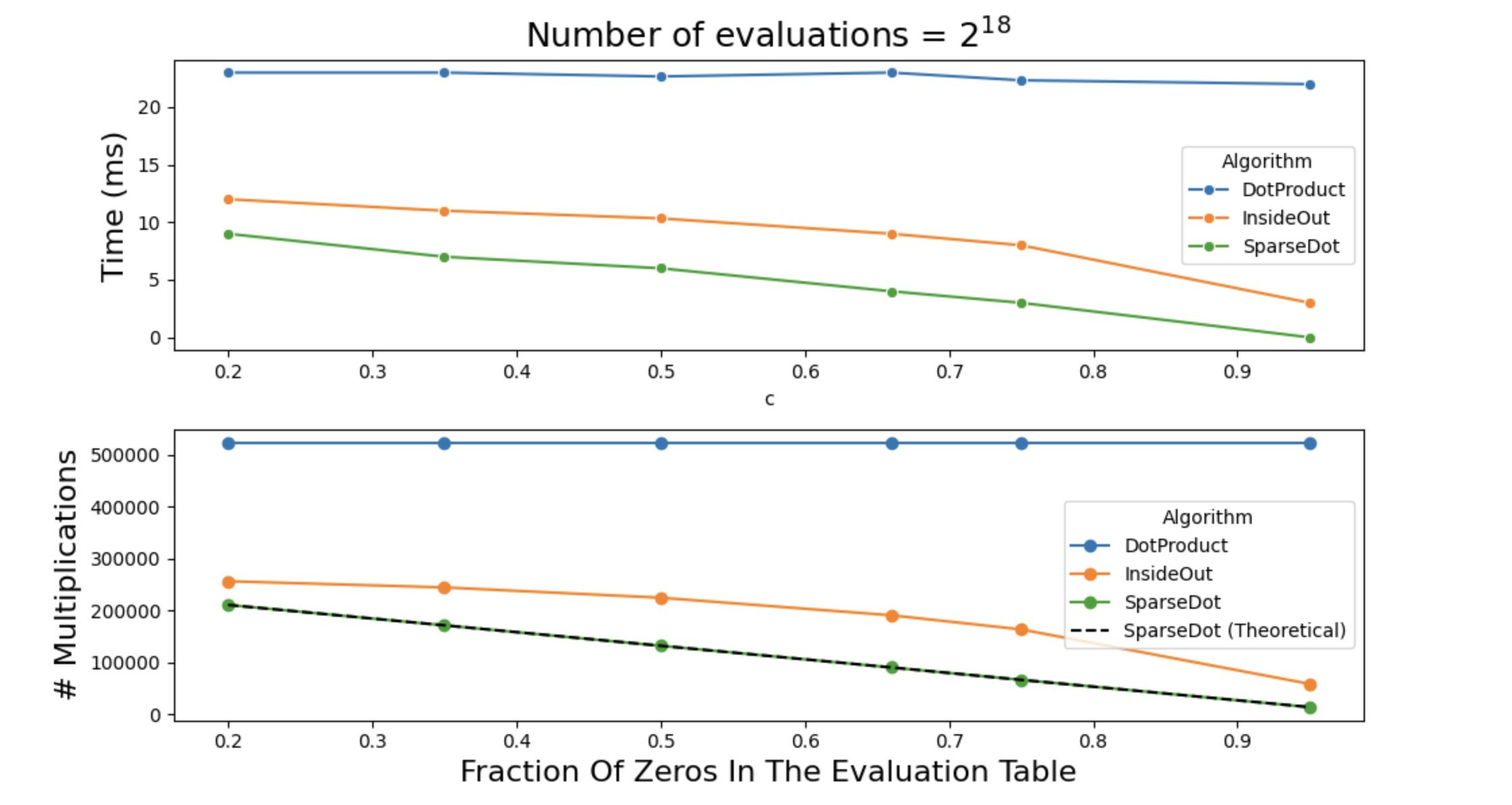
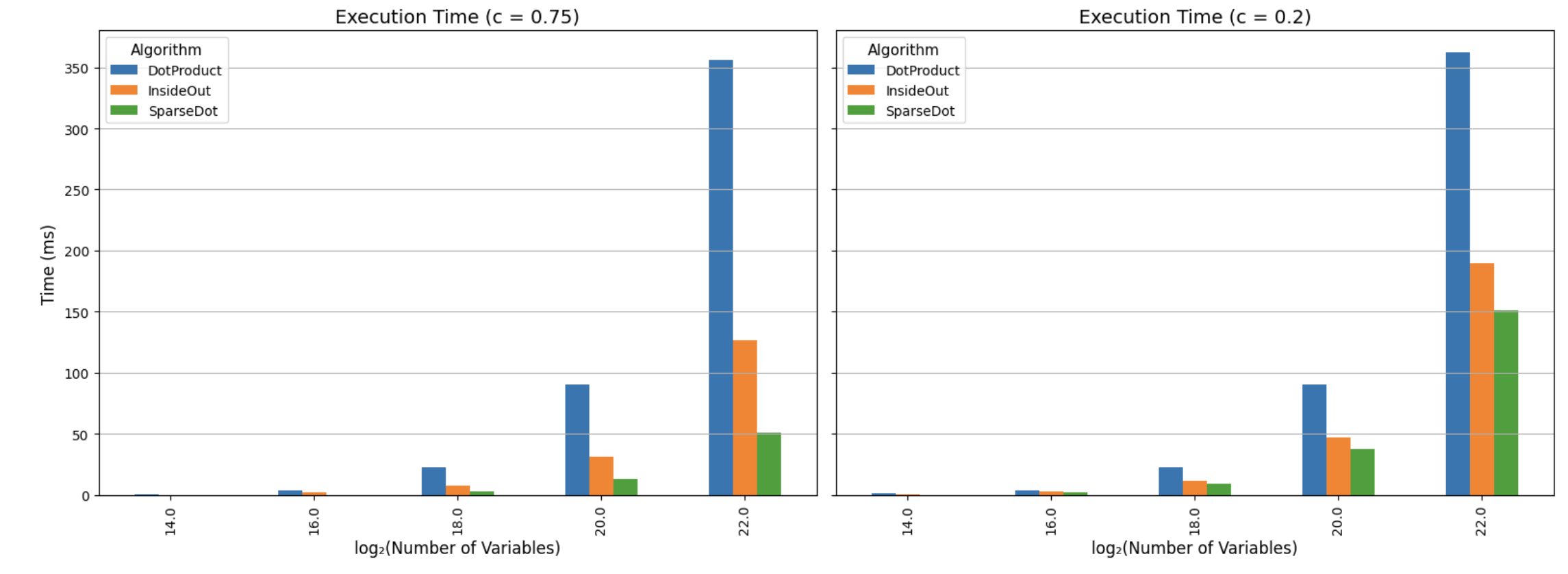
The plot below shows the physical times. We use Tracked Types to count the exact number of multiplications being done, and the dotted line describes what we expect to see in theory (as a sanity check for inefficiencies).
Notice how the two trends are almost identical, which does confirm that the bottleneck in polynomial evaluation really is field multiplication.
#TODO: Make these SVGS so they look better.
cargo run -p jolt-core --example polynomial_evaluation --release
Batched Polynomial Evaluation
Now we get to batched evaluations, that is we want to evaluate multilinear polynomials \(f_1, \ldots, f_s\) at the same point \(\vec{z}\).
Now the cost of computing \(eq\) is not as bad as it can be re-used for all \(\{f_i\}_{i \in [s]}\). Still we show splitting \(eq\) into \(eq_1\) and \(eq_2\) can provide time savings.
Once again we will measure both the exact number of multiplications, and the actual time it took to multiply things.
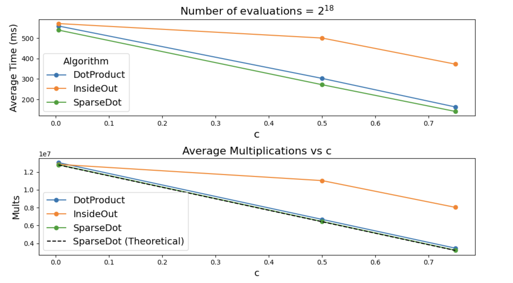
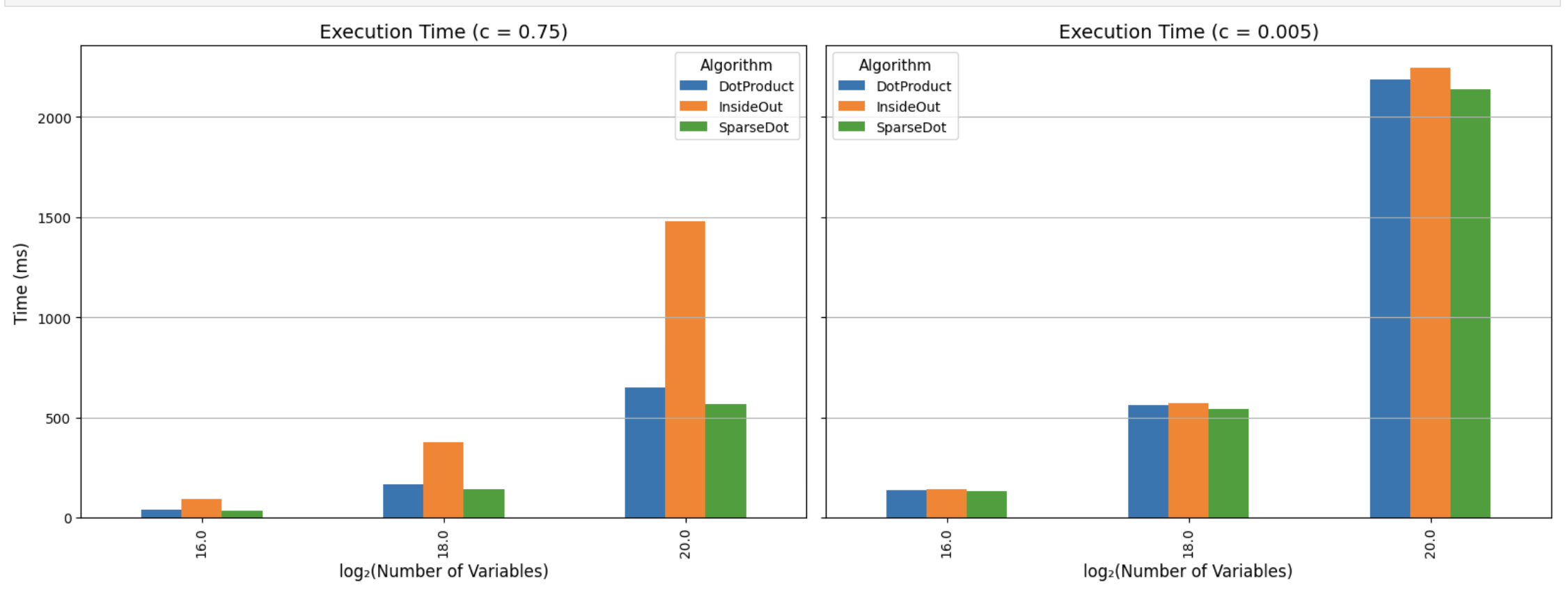
To get these plots run
cargo run -p jolt-core --example polynomial_evaluation --release
## References