Advent Of Jolt (Day 4): The Spartan Sumchecks
I must admit this took me longer to parse than I expected, and there are parts I’m still a little unsure about. There have been some major API changes since I started this. I’ll resume these soon, once the API has been consolidated post streaming sumchecks
On day 3 we went over all the constraints that must be satisfied. The way the prover convinces a verifier that it satisfied all these constraints (and, consequently proves they executed the trace faithfully), is via the sum-check protocol.
Jolt has a lot of sumchekcs as illustrated in the figure below. TODO:
In this post we focus on the sumchecks highlighted in green, tagged as Spartan Sumchecks. In subsequent posts we will handle the remaining sumchecks.
Stage 1 : The Outer Sum Check
Remember the 19 R1CS
constraints we discussed earlier. We add all zeros constraint to
make them a total of 20 constraints. Then we can index then using two
digits \((b,y)\) where \(b \in \{ 0, 1\}\), and \(y\in \{-5, \ldots, 4\}\). We choose those
indices for \(y\) instead of bit string
or the set \(\{0, \ldots, 9\}\) for
computational reasons, the details of which we dot discuss here (maybe
for a separate post). For each time step t we can write
these constraints as tables which in Jolt we refer to as
SpartanAz and SpartanBz, which we refer to
with \(A\) and \(B\) for brevity. The picture for \(A\) is the following:

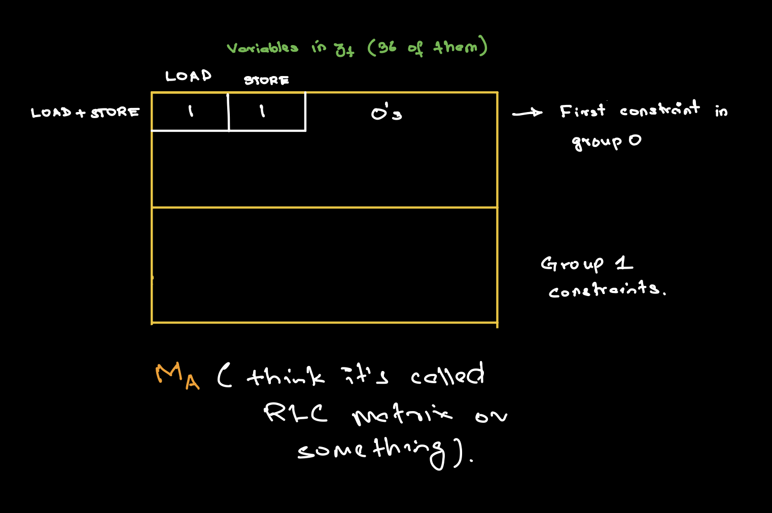
Recall that the first constraint looked like the following:.
(Load + Store) * (RamAddress - (Rs1Value + Imm)) = 0In table language we write for this time step \(t\):
A[t,0,-4] = z_t[LOAD] + z_t[STORE] and
B[t, 0, -4] = (RamAddress - (Rs1Value + Imm)).
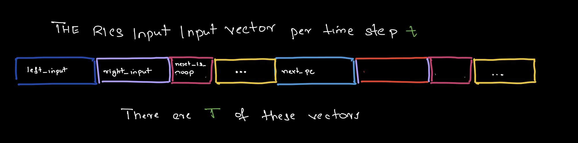
where was z_t above is the R1CSInput struct
we described on day 3. The mental
picture for z_t is the following:
Now satisfying all constraints is just saying the following:
\[\widetilde{A}(t, b, y) \otimes \widetilde{B}(t, b, y) = \vec{0} \quad \forall t \in \{0,1\}^{\log T}, \forall b \in \{0,1\}, \forall y \in \{-4, ..., 5\}\]
where \(\widetilde{A}, \widetilde{B}\) is the multi-linear extension of the Spartan \(A\) and \(B\) vectors, and \(\otimes\) represents the Hadamard product.
Now we do the thing we have done since the beginning of time. We want to make sure the LHS of the above system of equations to equal the RHS as polynomials. So we sample \((\tau_{\text{cycle}}|| \tau_b|| \tau_y) \xleftarrow[]{\$}\mathsf{C}^{\log T+2}\) and check if the following sumcheck holds:
\[\sum_{t \in \{0,1\}^{\log T}} \sum_{b \in \{0,1\}} \sum_{y \in \{-4,...,5\}} \widetilde{\mathsf{eq}}\left(\tau_{\text{cycle}}, t \right) \cdot \widetilde{\mathsf{eq}}\left(\tau_b, b \right) \cdot \mathcal{L}_{y}\left(\tau_y \right) \cdot \widetilde{A}(t, b, y) \widetilde{B}(t, b, y)\]
There are some implementation details where we handle the first round specially, but let’s ignore that for now. At the end of this sum-check the verifier must be able to open
\(\widetilde{A}(r_{\text{cycle}}, r_{b}, r_{y})\cdot \widetilde{B}(r_{\text{cycle}}, r_{b}, r_{y})\) but we don’t actually commit to \(\widetilde{A}\) and \(\widetilde{B}\). We say these are virtual. That is we will open something else later that is actually committed to. If the prover did that open honestly, then we open \(\widetilde{A}\) and \(\widetilde{B}\) as well (with high probability).
And that’s all there is to STAGE 1.
At the end of stage 1, we cache a bunch of other openings. Each field
in z has \(T\) values one
for each time step. For example, the field LeftInput has
\(T\) values, and we store \(\widetilde{\text{LeftInput}}(r_{\text{cycle}},
r_{b}, r_{y})\). We store the openings for all 36 fields.
Stage 2
Now we deal with two sumchecks ProductVirtual and
InnerSumcheck. The first sumcheck validates the product constraints we
discussed earlier. There’s an optimisation here where 5 checks are fused
into 1 check, but beyond that everything is quite similar to the outer
step.
Product Virtual Sumcheck
For all time steps \(t \in \{ 0, 1\}^{\log T}\) we want the following:
\[\begin{align} \text{LeftInstructionInput}(t) \cdot \text{RightInstructionInput}(t) &= \text{Product}(t) \\[10pt] \text{IsRdNotZero}(t) \cdot \text{WriteLookupOutputToRDFlag}(t) &= \text{WriteLookupOutputToRD}(t) \\[10pt] \text{IsRdNotZero}(t) \cdot \text{JumpFlag}(t) &= \text{WritePCtoRD}(t) \\[10pt] \text{LookupOutput}(t) \cdot \text{BranchFlag}(t) &= \text{ShouldBranch}(t) \\[10pt] \text{JumpFlag}(t) \cdot (1 - \text{NextIsNoop}(t)) &= \text{ShouldJump}(t) \end{align}\]
Sampling a random \(r_{\text{cycle}}\xleftarrow[]{\$}\mathsf{C}^{\log
T} \subset \mathbb{F}^{\log T}\) from the challenge set, we get
the following 5 separate sumchecks involving virtual polynomials (which
verify R1CS constraints where the Cz term is non-zero,
unlike the 19 constraints
discussed earlier).
Remark: \(r_{\text{cycle}}\) below is the exact same verifier random samples used in the Stage 1 sumchecks.
\[\begin{align} \sum_{t \in \{ 0, 1\}^{\log T}} \widetilde{\mathsf{eq}}\left(r_{\text{cycle}}, t \right) \cdot \text{LeftInstructionInput}(t) \cdot \text{RightInstructionInput}(t) &= \text{Product}(r_{\text{cycle}}) \\[10pt] \sum_{t \in \{ 0, 1\}^{\log T}} \widetilde{\mathsf{eq}}\left(r_{\text{cycle}}, t \right) \cdot \text{IsRdNotZero}(t) \cdot \text{WriteLookupOutputToRDFlag}(t) &= \text{WriteLookupOutputToRD}(r_{\text{cycle}}) \\[10pt] \sum_{t \in \{ 0, 1\}^{\log T}} \widetilde{\mathsf{eq}}\left(r_{\text{cycle}}, t \right) \cdot \text{IsRdNotZero}(t) \cdot \text{JumpFlag}(t) &= \text{WritePCtoRD}(r_{\text{cycle}}) \\[10pt] \sum_{t \in \{ 0, 1\}^{\log T}} \widetilde{\mathsf{eq}}\left(r_{\text{cycle}}, t \right) \cdot \text{LookupOutput}(t) \cdot \text{BranchFlag}(t) &= \text{ShouldBranch}(r_{\text{cycle}}) \\[10pt] \sum_{t \in \{ 0, 1\}^{\log T}} \widetilde{\mathsf{eq}}\left(r_{\text{cycle}}, t \right) \cdot \text{JumpFlag}(t) \cdot (1 - \text{NextIsNoop}(t)) &= \text{ShouldJump}(r_{\text{cycle}}) \end{align}\]
The RHS of these equations were stored from virtual openings.
Instead of 5 separate sumchecks, create polynomials \(l(t, z)\) and \(r(t, z)\) such that:
\[\begin{align} \text{At } z = -2: \quad & l(t, -2) = \text{LeftInstructionInput}(t), \quad r(t, -2) = \text{RightInstructionInput}(t), \quad p(t, -2) = \text{Product}(t) \\[10pt] \text{At } z = -1: \quad & l(t, -1) = \text{IsRdNotZero}(t), \quad r(t, -1) = \text{WriteLookupOutputToRDFlag}(t), \quad p(t, -1) = \text{WriteLookupOutputToRD}(t) \\[10pt] \text{At } z = 0: \quad & l(t, 0) = \text{IsRdNotZero}(t), \quad r(t, 0) = \text{JumpFlag}(t), \quad p(t, 0) = \text{WritePCtoRD}(t) \\[10pt] \text{At } z = 1: \quad & l(t, 1) = \text{LookupOutput}(t), \quad r(t, 1) = \text{BranchFlag}(t), \quad p(t, 1) = \text{ShouldBranch}(t) \\[10pt] \text{At } z = 2: \quad & l(t, 2) = \text{JumpFlag}(t), \quad r(t, 2) = (1 - \text{NextIsNoop}(t)), \quad p(t, 2) = \text{ShouldJump}(t) \end{align}\]
Define \(S = \{-2, -1, 0, 1, 2\}\).
Now if we wanted to check all 5 constraints are satisfied, we simply check1:
\[\sum_{t \in \{ 0, 1\}^{\log T}} \widetilde{\mathsf{eq}}\left(r_{\text{cycle}}, t \right) \sum_{z \in S} \cdot \mathcal{L}_{z}\left(\tau \right) \cdot \ell(t,z) \cdot r(t,z) = \sum_{z \in S} \mathcal{L}_{z}\left(\tau \right) \cdot p(r_{\text{cycle}}, z)\]
The Inner Sumcheck
This uses information from outer sumcheck. In particular we re-use
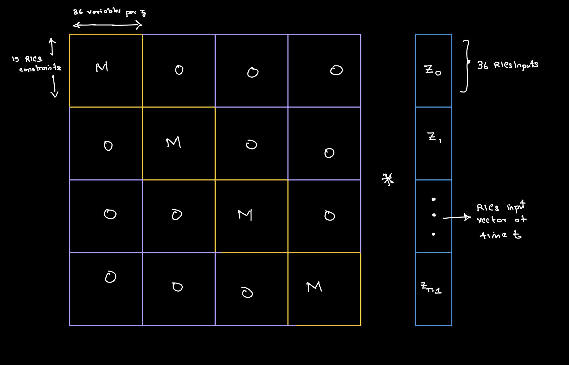
\(r_{\text{cycle}}, r_{b}\) and \(r_{y}\) from stage 1. Let \(C\) be the number of fields the
z_t the R1CSInput struct has. The Outer
sumcheck guarantees that we the constraints are satisfied, assuming
\(A\) and \(B\) were properly formed. What’s stopping
me from setting \(A\) and \(B\) to all zeros and satisfying the
sumcheck? How do I prove that I actually used \(z_t\) to construct the rows of
SpartanAz and SpartanBz? The following
sumcheck essentially guarantees that SpartanAz is correctly
constructed (assuming z was correctly constructed). We will
get to z’s correctness later (for now assume it is so).
\[\begin{align} \sum_{z \in \{ 0, 1\}^{\log C}} \Big( \widetilde{M_A}[r_{b}, r_{y}, z]\cdot \widetilde{z}[r_{\text{cycle}}, z] + \gamma\cdot \widetilde{M_B}[r_{b}, r_{y}, z]\cdot \widetilde{z}[r_{\text{cycle}}, z] \Big) = {} & \\ \widetilde{A}[r_{\text{cycle}}, r_{b}, r_{y}] + \gamma\,\widetilde{B}[r_{\text{cycle}}, r_{b}, r_{y}]. \end{align}\]
where \(\gamma \xleftarrow[]{\$}\mathsf{C}\), and the mental model for \(M_A\) (and \(M_B\)) similarly is the following:
 and zooming in
Stage 3 Sumchecks
ShiftSumcheck
let shift_sumcheck = ShiftSumcheckProver::gen(state_manager, key);
InstructionInputSumcheck
let instruction_input_sumcheck = InstructionInputSumcheckProver::gen(state_manager);
ProductVirtualInner
let product_virtual_claim_check = ProductVirtualInnerProver::new(state_manager);
The actual code uses split eq poly optimization from Gruen.↩︎