Remaining Task list
- Chi-Squared Test notes
- Uniqueness private notes: This comes for free if you understand the non private one
- Collisions private notes
- Uniqueness non-private notes
- Goldreich Generalisation (I’ll do this in a bit – bucketing/discretisation)
- LDP notes for Chi Squared Test (Acharya et al., 2019), (Acharya et al., 2020) and (Acharya et al., 2021)
- How does the sample complexity change under shuffle privacy Uniformity Testing in the Shuffle Model: Simpler, Better, Faster
Summary
In this document, we only deal with discrete distributions over the simplex of size k. The papers referenced below derive results for continuous analogues wherever appropriate. The goal is to try and understand differentially private distribution testing. Naturally, to understand DP-testing, we first need to understand non-private testing. It is possible that I have made typographic errors or other minor errors.
| Uniformity Testing | |
|---|---|
| Non-Private1 | \theta(\frac{\sqrt{k}}{\eps^2}) |
| Central DP2 | O(\frac{\sqrt{k}}{\eps^2} + \frac{\sqrt{k}}{\eps \sqrt{\varepsilon}}) |
| Shuffle DP3 | O\Bigg(\frac{k^{3/4}}{\eps\varepsilon}\sqrt{\ln \frac{1}{\delta}} + \frac{\sqrt{k}}{\eps^2}\Bigg) |
| LDP4 | \theta(\frac{k^{3/2}}{\eps^2\varepsilon^2}) |
Introduction
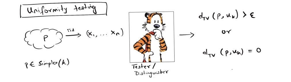
A testing algorithm \mathcal{T} sees n i.i.d samples from unknown distribution \bvec{p} \in \simplex{k} and based on those observations it wants to decide if \bvec{p} is the uniform distribution i.e. \bvec{p}=\bvec{u}_k or p is \eps-far away from the uniform distribution i.e. d_{TV}(\bvec{p}, \bvec{u_k}) \geq \eps, where d_{TV}(X, Y) = \frac{1}{2}||X - Y||_1 refers to the total variation distance between two discrete distributions X and Y.
If p=U_k (accepting), the tester outputs \mathcal{T}(x_1, \dots, x_n) = 0 and \mathcal{T}(x_1, \dots, x_n) = 1 otherwise (rejecting). The figure below illustrates the idea.
We’d like \mathcal{T}’s guess to be correct with a probability greater than equal to \frac{2}{3} (though this can be amplified to arbitrary \delta with \ln 1/\delta more samples).
Instead of \bvec{u}_k if we had picked an arbitrary \bvec{q} \in \simplex{k} to test against, the problem is referred to as identity testing. (Goldreich, 2016) show a transformation that shows that if we can solve uniformity testing, then we can solve the identity testing for generic \bvec{q} \in \simplex{k} as well i.e. uniformity testing is complete. see my notes. Thus the focus of this document is mostly restricted to uniformity testing.
Non-Private Testers
One cannot analyse differentially private testers without understanding how to solve the simpler problem first. In this setting, the only source of randomness is the sampling procedure by which we see x_1, \dots, x_n where each x_i \in [k]. Recall that
\begin{equation} d_{TV}(\bvec{p}, \bvec{q}) = \frac{1}{2}|| \bvec{p} - \bvec{q} ||_1 \leq \frac{\sqrt{k}}{2}|| \bvec{p} - \bvec{p} ||_2 \end{equation}
where the last inequality comes from Cauchy-Schwartz (or equivalence of norms, however you call it).
Now if d_{TV}(\bvec{p}, \bvec{q}) \geq \eps, then \frac{\sqrt{k}}{2}||\bvec{p} - \bvec{u_k} ||_2 \geq \eps. Re-arranging we get ||\bvec{p} - \bvec{u_k} ||_2^2 \geq \frac{4\eps^2}{k} in the far away case and ||p||_2^2 = \frac{1}{k} in the uniform case. Our goal is to come with some test which looks at the data and comes up with a statistic T such that \E[T] is related to either ||\bvec{p} - \bvec{u_k}||_2^2 or ||\bvec{p} - \bvec{u_k}||_1. Then based on the magnitude of the value of \E[T] we can decide to \accept or \reject. The figure below illustrates the idea when T equals the fraction of pairwise collisions in the sample.
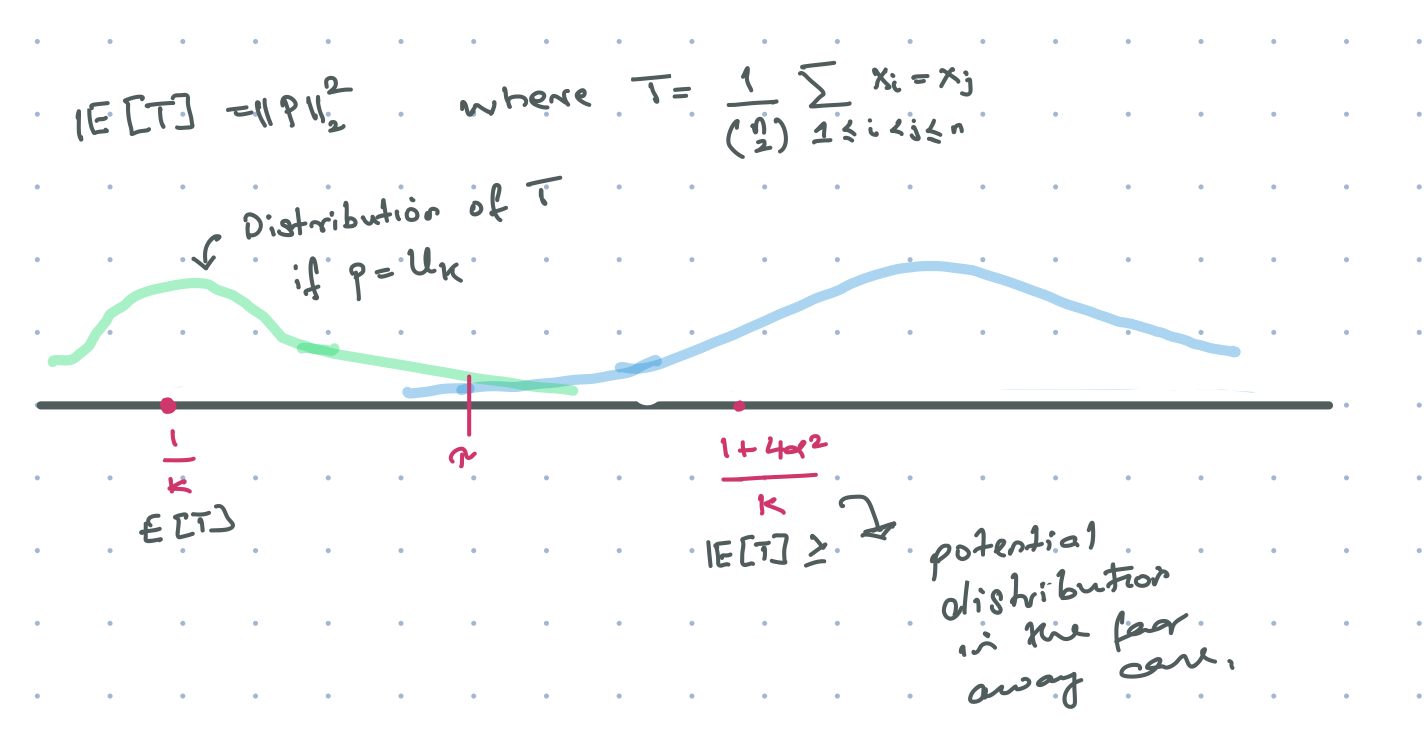
Of course there is one caveat – the variance of the estimate T should be much smaller than the expectation gap \Delta := \E_{x_i \sim \bvec{u_k}}[T] - \E_{x_i \sim \bvec{p}}[T] \ll \frac{4\eps^2}{k}. Otherwise all our claims based on the size of T are useless. So all proofs have uniformity testers have two steps:
- Relate the expectation of the test statistic to either || \cdot ||_1 or || \cdot ||_2^2.
- Show that the variance of the estimator smaller than the expectaion gap.
Next we describe two natural intuitive statistics. If a distribution is truly uniform, we do not expect to see too many samples take the same value. Two different ways of quantifying the overlap between samples is to count (1) collisions: the number of pairs of samples that are the same and (2) number of unique items in a sample of n items (clearly n \ll k for this to make sense).
When T is the number of pairwise collisions, it’s expectation is naturally related to ||\bvec{p} - \bvec{u_k}||_2^2. The only work we have to do is bound the variance, which comes with a little manipulation of binomial coefficients. For details see Non-private Collision Tester. On the other hand, it is not as easy to see how counting unique elements is related to the distance between two distributions. However, with a little help from calculus, we can show that the expectation gap between counts under the two distributions is directly related to the total variation distance. This observation gives rise to the Non-private Uniqueness Tester. In both of the documents, the bulk of the work is in upper bounding the variance of these estimators.
Another natural test to look at the empirical counts for each j \in [k] in the n samples and do a goodness of fit using a chi-squared test. Turns out this works out quite nicely too – Non-private Chi-Squred Tester.
Note: There are many other tests (as described in Chapter 2 of (Canonne, 2022)), but I have not had the time to go through them all. Of particular interest is the empirical distance tester which is Lipschitz, and thus lends itself very easily to differential privacy. Work to reference (Acharya et al., 2018).
Differentially Private Testers
Now that we somewhat understand how to do uniformity testing, we constrain the output of the test to be differentially private i.e. if we changed one of the samples from the stream of data, we don’t want the decision to change drastically. The problem is still the same – what is the sample complexity? As the output of the tester is \{ 0, 1\}, more formally we want our tester to satisfy the additional property of privacy along with being able to distinguish between two scenarios described in the non-private setting.
\begin{equation} \max\Big\{ \frac{\Pr[\mathcal{T}(X_1, \dots, X_n) = 1]}{\Pr[\mathcal{T}(X_1^\prime,\dots,X_n) = 1]}, \frac{1 - \Pr[\mathcal{T}(X_1, \dots, X_n) = 1]}{1 - \Pr[\mathcal{T}(X_1^\prime,\dots,X_n) = 1]} \Big\} \leq e^{\varepsilon} \end{equation}
It is not clear to me why this when it would be useful to this in a practical setting. I found the arguments in the introduction unsatisfying. Most papers started with the uniformity testing and then claimed described DP independently..
Remember the testing algorithms described above output a scalar statistic T. Then the test thresholds this statistic against some constant, say \tau and decide whether to \accept or \reject. Thus making the testing algorithm DP is equivalent to making the test statistic DP. The two standard ways to make any output DP is to either (1) Add noise to a statistic from a smooth distribution – laplace, gaussia, poisson, negative binomial, binomial etc. (2) Generate an output by some sampling procedure where the output probabilities are a function of test statistic. Examples include sub-sampling (Wang et al., 2019), sample and threshold (Bharadwaj and Cormode, 2021), exponential mehcanism (Dwork, 2008).
Turns out there is an algorithm for converting any non-private test to a differentially private test based on sub-sampling- Generic Tester. However, just like sampling is not asymptotically as good as additive noise from a laplace distribution in terms of privacy-accuracy tradeoff. Testers based on additive noise were shown by (Aliakbarpour et al., 2018) and (Acharya et al., 2018). It is unclear if this makes any difference in practice – I will have to write some code simulating all the use cases
(Aliakbarpour et al., 2018) takes the two classic non-private tests based on collisions and uniqueness and makes them DP by adding laplace noise. The uniqueness tester is easy, as the test statistic has small global sensitivity \Delta=1. So adding a \mathtt{Lap}(\frac{1}{\varepsilon}) to the non-private statistic makes it private. Then all there is to show is that via concentration lemmas, the variance of the noise is small enough where it doesn’t really affect the output of the statistic. See details below. However, all tests based on uniqueness are restricted to n \ll k, which might not always be practical for unless k is very large.
Private test based on uniqueness
Sample Complexity:= O(\frac{\sqrt{k}}{\eps^2} + \frac{\sqrt{k}}{\eps \sqrt{\varepsilon}})
Let Z_2 = \frac{1}{n}\sum_{j \in [k]} \unit(N_j = 1) be the empirical mean of the number of unique elements, where N_j = \sum_{j=1}^n \unit(X_j = i) for all j \in [k] is the count of elements. The test statistic Z_2 has very small global sensitivity. If two samples differ by 1 element then the number of unique samples differ by at most 2. Thus we have ||Z_2 - Z_2^\prime ||_1 \leq 2. This is just differentially private mean estimation with low sensitivity – adding Laplace noise with scale \frac{2}{\varepsilon} makes the statistic DP.
From the DP literature we know that this is smallest magnitude of noise we can add to get DP i.e. if we want Z_2 to be DP, we cannot do better.
Accuracy of private test based on uniqueness
The accuracy proof is nearly identical to the non-private uniqueness proof I derived the following results independently, but they are likely very similar to Appendix E of (Aliakbarpour et al., 2018). As the final bounds were the same, I did not bother checking.
Borrowing notation from non-private uniformity testing
Let Z_2 = \frac{1}{n}\sum_{j \in [k]} \unit(N_j = 1) be the empirical avereage of the number of unique observations out of n i.i.d samples, where N_j = \sum_{i=1}^n \unit(x_i = i) counts the number of occurrences for all j \in [k].
Recall uniformity testing can be broken down into 3 steps:
Show that the summary statistic in expectation is related to d_{TV}(\bvec{p}, \bvec{u_k}). We already did this in the non-private case (see here for a refresher). We showed that \mathbb{E}_{\bvec{u_k}}[Z_2] - \mathbb{E}_{\bvec{p}}[Z_2] \geq \frac{n}{16k}d_{TV}(\bvec{p}, \bvec{u_k})^2. Adding zero mean independent noise to this statistic does not change it’s expectation, just the variance. So all we have to show is that adding a little bit of Laplace noise, did not change the variance by that much.
Bound the variance of the estimator and show that it does not exceed the expectation gap. Note the \frac{1}{n}\Big(\mathtt{Laplace}(\frac{2}{\varepsilon})\Big) noise is independent of x_1, \dots, x_n. Therefore, by linearity we could just add the non-private variance with the additional variance to get the upper bound. The variance is is just \frac{8}{n^2\varepsilon^2}. The rest follows easily. Let \tilde{Z_2} = Z_2 + \frac{1}{n}\mathtt{Lap}(\frac{2}{\varepsilon}). In the uniform case we have
\begin{align} \Pr{\Bigg[ \tilde{Z_2} \leq \tau \Big| d_{TV}(p, U_K) = 0 \Bigg]} &= \Pr{\Bigg[ \tilde{Z_2} \leq \mathbb{E}_{\bvec{u_k}}[\tilde{Z_2}] - \frac{\Delta}{2} \Bigg]} \\ &\leq \frac{4\var[\tilde{Z_2}]}{\Delta^2} \\ &\leq \frac{c_1k}{n^2\eps^4} + \frac{c_2k^2}{n^4\eps^4\varepsilon^2} & \leq \frac{1}{3} \end{align}
In the far away case, the argument is once again the same. Borrowing from non-private uniformity testing we have
\begin{align} \Pr{\Bigg[ \tilde{Z_2} \geq \tau \Big| d_{TV}(p, U_K) \geq \eps \Bigg]} &= \Pr{\Bigg[ \tilde{\tilde{Z_2}} \geq \mathbb{E}_{\bvec{u_k}}[\tilde{Z_2}] - \frac{\Delta}{2} \Bigg]} \\ &= \Pr{\Bigg[ \tilde{Z_2} \geq \mathbb{E}_{\bvec{p}}[\tilde{Z_2}] + \Delta(p) - \frac{\Delta}{2} \Bigg]} \\ &= \Pr{\Bigg[ \tilde{Z_2} \geq \mathbb{E}_{\bvec{p}}[\tilde{Z_2}] + \frac{\Delta(p)}{2} + \frac{\Delta(p)}{2} - \frac{\Delta}{2} \Bigg]} \\ &\leq \Pr{\Bigg[ \tilde{Z_2} \geq \mathbb{E}_{\bvec{p}}[\tilde{Z_2}] + \frac{\Delta(p)}{2} \Bigg]} \\ &\leq \frac{4\var[\tilde{Z_2}]}{\Delta(p)^2} \\ &\leq 4\Big(\frac{c_1}{k\Delta(p)^2} + \frac{c_2}{n\Delta(p)} + \frac{c_3}{n^2\varepsilon^2\Delta(p)^2}\Big) \\ &\leq 4\Big(\frac{c_1}{k\Delta^2} + \frac{c_2}{n\Delta} + \frac{c_3}{n^2\varepsilon^2\Delta^2}\Big) \\ &\leq \frac{1}{3} \end{align}
Plugging \Delta:= O(\frac{n\eps^2}{k}) does the job. Solving for n we get n \geq O(\frac{\sqrt{k}}{\eps^2} + \frac{\sqrt{k}}{\eps \sqrt{\varepsilon}}) for both cases.
Private test based on collisions
The statistic that counts number of pairwise collisions has global sensitivity that grows O(n) instead. The authors note that the sensitivity is a function of the most frequent element in the sample. However if any particular element occurs very frequently, then 1) The global sensitivity is high 2) The distribution is very likely not uniform. So a way to reduce the global sensitivity is to just clip the most frequent item and then do the test. This reduces the sensitivity of the test and we get DP by adding a little bit of Laplace noise. It proof is a little bit more elaborate but the core ideas are pretty standard to DP mean estimation when the size of the domain is quite big. For details see below.
Sample complexity := \Theta\Big(\frac{\sqrt{k}}{\alpha^2} + \frac{\sqrt{k\max(1, \ln 1/\varepsilon)}}{\alpha\varepsilon} + \frac{\sqrt{k\ln k}}{\alpha\varepsilon^{1/2}} + \frac{1}{\varepsilon\alpha^2}\Big) I have no idea how worse this is from the generic tester in practice, will need to code up
Given n i.i.d samples X_1, \dots, X_n let Z_1 = \frac{1}{\binom{n}{2}}\sum_{1 \leq s < t \leq n} \unit(X_s = X_t) be the empirical average fraction of collisions in the dataset. The test statistic Z_1 has very high sensitivity. If two samples differ by just 1 element the number of pairwise collisions can change by n. Thus it is no good adding Laplacian noise with scale \frac{n}{\varepsilon}. We will get DP but the test would become completely useless. As a workaround, there is a pre-processing step.
Note that sensitivity of Z_1 depends on the maximum number of occurrences of an item. Let N_j denote the count of item j \in [k] in the sample X_1, \dots, X_n and N_{\max} = \max_{i \in [k]}N_j is the sensitivity of Z_1 on two neighbouring datasets. If N_{\max} is really high, we would need a lot of noise, but it is also unlikely that the data is sampled from the uniform distribution. Why ? See the following lemma:
Source: Lemma F.2 (Aliakbarpour et al., 2018).
Let x_1, \dots, x_n represent n i.i.d samples from \bvec{u_k}. Let N_j be the observed count of element j \in [k]. Define N_{\max} := \max_{j \in [k]}N_j. We have with probability \frac{23}{24} that
\begin{equation} N_{\max} \leq \max\Big\{ \frac{3n}{2k}, 12e^2\ln(24k)\Big\} \end{equation}
Thus pick a threshold \tau_1 = \max\Big\{ \frac{3n}{2k}, 12e^2\ln(24k)\Big\} and if N_{\max} is greater than that threshold, always reject the hypothesis. The global sensititvity of N_{\max} is just 2. And since we will use this $N_{} to make a decision whether to accept or reject, we will need to privatise it with \mathtt{Laplace}(\frac{2}{\varepsilon}). From the tail bounds of Laplace distributiosn we have that
\begin{equation} \Pr\Bigg[\mathtt{Lap}(\frac{2}{\varepsilon}) \geq \frac{2\ln12}{\varepsilon}\Bigg] \leq \frac{1}{24} \end{equation}
Combining this with the Lemma above we have the differentially private \tilde{N}_{\max} = N_{\max} + \mathtt{Lap}(\frac{2}{\varepsilon}) \leq \max\Big\{ \frac{3n}{2k}, 12e^2\ln(24k)\Big\} + \frac{2\ln12}{\varepsilon} with probability \frac{11}{12}.
Define \eta_f = \max\Big\{ \frac{3n}{2k}, 12e^2\ln(24k)\Big\} + \frac{2\ln12}{\varepsilon} which is a probabilistic upper bound on \N_{\max}. If \N_{\max} \geq \eta_f – output \reject always (and we would be correct very often). So the only interesting case we have is when \N_{\max} \leq \eta_f, in this case we cannot just output \accept. We still need to look at the pairwise collisions which we know is an optimal statistic. But now the sensitivity of the Z_1 in this clipped setting is just \eta_f, which is a function of \ln k instead of O(n) as compared to the unclipped setting. So now the noise is \mathtt{Lap}(\frac{\eta_f}{\varepsilon}) which of course would affect the variane of the collisions estimator.
The final derivation of the sample complexity follows from Lemma F.1 of (Aliakbarpour et al., 2018) which shows that the additional cost of this laplace noise is \Theta\Big(\frac{\sqrt{k\max(1, \ln 1/\varepsilon)}}{\alpha\varepsilon} + \frac{\sqrt{k\ln k}}{\alpha\varepsilon^{1/2}} + \frac{1}{\varepsilon\alpha^2}\Big)
Tester observers noisy sample (LDP)
Another privacy variant for the same problem is to ask, the same questions but when the samples have been passed through a local randomiser before being sent to the testing algorithm. (Acharya et al., 2019) provide optimal sample complexity results for samples that are randomised by Rappor and the Hadamard transform. It is known that randomised response generalises all LDP protocols, so an upper bound on uniformity testing for Rappor, gives us a sample complexity upper bound for LDP in general.
Here they show that the due to the more noise accepted by local randomisers, the collisions based tester is no longer optimal. They have to rely on the chi-squared tester from the non-private world5.
Claim: Public coin protocols take far fewer samples than private coin protocols. Unsure – why!!
Question: We know dishonest users can completely ruin the utility of estimation but does dishonesty make sense from a testing perspective?
Follow up work (Acharya et al., 2020) and (Acharya et al., 2021): Have not read
Shuffle Privacy and it’s implications
Finally, the same questions are asked under shuffle privacy, when the samples have been passed through a local randomiser such that collectively the samples are differentially private. As the level of noise is lower, we expect the sample complexity to be better than LDP. See Uniformity Testing in the Shuffle Model: Simpler, Better, Faster. I have not read this paper at all.
Questions
- Posed by Varun Jog: For simple hypothesis testing, what happens when the samples have been passed through a local randomiser instead. How is the sample complexity affected ?
- Posed by Graham: Is there a master theorem or master lemma that covers all the theorems I have surveyed – can we say something general about DP outputs of a class of functions that are not too bad. Maybe all test statistics belong to this not too bad set of functions.
- Do not have a great sense for why some tests are worse than others when dealing with private testing. For example why is Chi-Squared test robust to LDP perturbation but the uniqueness tester is not.
References
Collission tester, uniqueness tester or chi-squared tester, they all have the same sample complexity. Not sure which ones work better in practice.↩︎
Based on the uniqueness tester.↩︎
What trick do they use? TODO.↩︎
Based on the chi-squared tester.↩︎
I must admit I have a really hard time with these moment generating function proofs and chi-squared business. It’s not as intuitive as counting things. But I have to do understand them nevertheless. TODO.↩︎