Simple Hypothesis Testing
Sample Complexity: How many i.i.d samples must I observe to be fairly confident to guess with the abovementioned confidence?
As expected, the number of samples needed is a function of how close the two distributions are, where closeness is measured using Hellinger Distance. Defining some notation– Let n(\mathcal{P}) be the sample complexity to distinguish distributions in \mathcal{P} with a probability of error less than one-third. Then for \mathcal{P}=\{p, q\} where p,q are members of some family of probability distributions \mathcal{P} we have
\begin{equation} n(\mathcal{P}) = \theta\Bigg(\frac{1}{d_{H}(p,q)^2}\Bigg) \end{equation}
See section 1 of this document for full proof derivation.
Jupyter notebook simulation to see if the above claims are meaningful
Private Hypothesis Testing
Based on the works of (Canonne et al., 2019). Now say we wanted to do all of the above things but wanted the output of the hypothesis test to be private. Let \mathcal{A} be the algorithm that decides whether samples X_n is from p or q. If \mathcal{A}(X_n)=1, we conclude the data was sampled from p, otherwise, if \mathcal{A}(X_n)=0, we claim the data was sampled from q. For the output \mathcal{A} to be (\eps, \delta) DP, we must have had with probability 1 - \delta that
\begin{equation} \max\Big\{ \frac{\Pr[\mathcal{A}(X_n) = 1]}{\Pr[\mathcal{A}(X_n^\prime) = 1]}, \frac{1 - \Pr[\mathcal{A}(X_n) = 1]}{1 - \Pr[\mathcal{A}(X_n^\prime) = 1]} \Big\} \leq e^{\eps} \end{equation}
where X_n, X_n^\prime
Now say we are sampling from p, and we see a sample x_n was unlikely to be seen i.e. it is extremely unlikely over p but likely over q. In the non-private setting, \mathcal{A} is free to change its mind and claim this dataset did indeed come from q. In the private setting, one data point we restrict \mathcal{A} such that it cannot change its output so easily. Thus private hypothesis testing appears to be equivalent to robust hypothesis testing (or stability-based hypothesis testing).
Sample Complexity: What effect does imposing this privacy constraint have on the sample complexity –[TODO]
Key results
- If \eps is large enough i.e. the privacy constraint is not too strict, then this restriction makes no real difference i.e. when \eps \geq \max_{x \in [k]} \Bigg| \ln \frac{p(x)}{q(x)} \Bigg| we have
\begin{equation} n_{\eps}(\mathcal{P}) = \theta\Bigg(\frac{1}{d_{H}(p,q)^2}\Bigg) \end{equation}
Hypothesis Testing Under Communication Constraints
Now suppose the distinguisher \mathcal{A} has very limited bandwidth channel via which it observes this independent samples. It can no longer see x_i in clear but instead sees x_i discretised to 1 out of D values for all i \in [n]. Thus their inputs must be discretised into one of the values in set D = \{1 , \dots, D \}.
Now the task is to come up with an efficient discretising (compression) algorithm T: [k] \rightarrow [D] and then have A distinguish between p and q based on T(x_1), \dots, T(x_n).
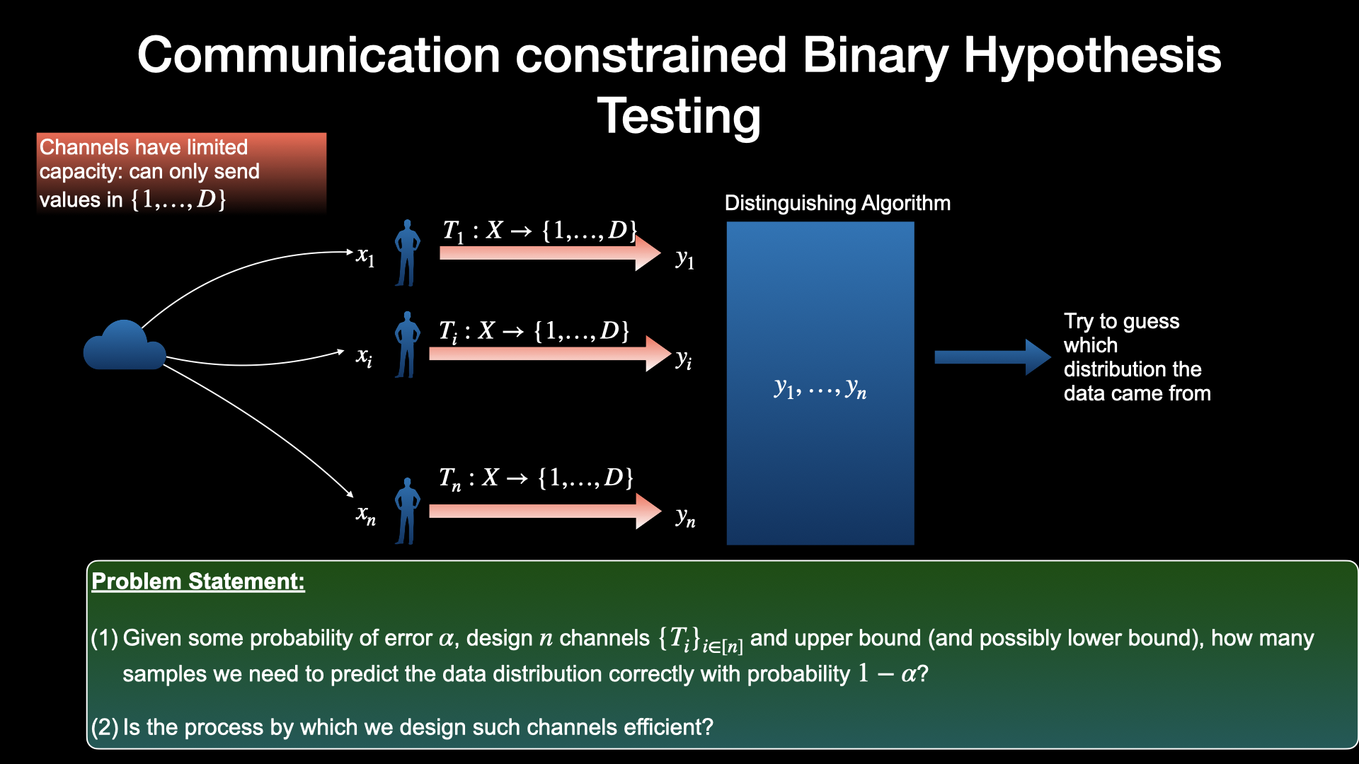
Sample Complexity: The questions posed in the illustration above are answered by (Pensia et al., 2022)
Key results
They key results can be described as follows:
Let n_D(P) be the sample complexity for distinguishing distributions in \mathcal{P} when the distinguisher observes discretised inputs as described above. Then the authors come up with a set of channels and distinguishing algorithm such that
- n_D(P) \leq n(P)\max(1, \frac{\ln n(P)}{D}) i.e. we only need a log factor more samples
- Furthermore, there exist cases where the bound is tight. (what cases?)
See section 2 of this document for my re-derivations of the key results
LDP Hypothesis Testing
Now instead of discretised samples, if we observed samples that have passed through a local randomiser. How does the sample complexity change?
This is open